Chapter I- Lesson 1 of 1 Transient and Harmonic Analysis (of Linear Systems)
Instructions
- Read the lecture (displayed below) [30-60 minutes]
- Watch the video (10:30 minutes) [30 minutes]
- Do the exercises [~30 minutes]
Total time = [~2:00 hours]
Lesson 1 of 1
: Transient and Harmonic Analysis (of Linear Systems)
- In This Chapter (Overview of Chapter Contents and Important Highlights)
- Time Domain and Frequency Domain
- States and Languages
- Phasors and Frequency Domain (Harmonic) Analysis
- Use of Phasors in Circuit Analysis (in the Frequency Domain)
- Demonstration of Circuit Analysis in the Frequency Domain
- The Frequency Domain and the Laplace Transform
- Addendum: The Mystery of $j$ and Imaginary Numbers
Introduction:
We live in the time domain… All occurrences happen in the time domain... Events happened in the past… happen in the present… and other events will happen in the future…! We witness physical phenomena in the real world and express their properties in real numbers. However, at times, we use imaginary tools and fictitious descriptions to facilitate the analysis, especially in difficult physical situations.
Much of this is true in our electrical engineering studies. Examples of imaginary tools are the use of complex variables to describe voltage phasors, impedances, and complex power. Examples of fictitious (nonphysical) descriptions include non‐causal operations, integrations from zero to infinity, and “steady state” harmonic analysis.
With this introduction, you may think that this book intends to discredit the foundation of all our electrical engineering education and more. The answer is “nope”. What is intended here is to remind the reader of some “basic” foundations that get overlooked with time and raise relevant warning flags. It is important that we stay mindful of the foundations used in developing the tools that we constantly use and apply. In addition, it is most important to be aware of the physics of all procedures we carry out and tools we use.
Our subject in this chapter is Transient and Harmonic Analyses… Transient analysis deals with the system (or circuit) response to a time varying excitation during the transition between two steady states. One example is the famous battery‐switch‐RC circuit when we throw the switch on or off to charge or discharge the capacitor. Another example would be studying the transient as we turn on (or off) an AC (110/220 V 50/60 Hz) appliance.
The other type of analysis we refer to here is what we call harmonic analysis and there is a good reason for choosing this wording over other familiar wordings…! You see… the complementary state to transient is “steady”. However, steady may mean steady constant or steady variable, i.e. periodic. Considering steady constant as a special case of periodic with a period that is too long (mathematically, we say infinite), then we can identify the alternate state to transient as the “periodic” one, the simplest form of which is the harmonic time variation. Also, noting that for linear systems, the Fourier analysis can enable us to express other forms of periodic variations as a superposition of harmonics of different periodicities (different frequencies). Hence, we can claim that by covering transient and harmonic analyses, we are in fact covering tools that can encompass all forms of linear system analyses that we can think of.
Time Domain and Frequency Domain:
Now, we have two possible domains that we can work in; the time domain and the frequency domain. The time domain is where we deal with all analysis procedures as functions of time. In this type of analysis, we typically develop time dependent differential equations to express the behavior of physically based system (or circuit) models. Solving these equations can get too complicated and we may end up resorting to mathematical procedures and transforms to enable a solution. One typical transform that we often use in solving electrical circuit problems in the time domain is the Laplace transform. The Laplace transform converts the time derivatives into powers of “s” in a complex “s” domain and we end up with algebraic equations that are typically solvable. Once we get a solution in the “s” domain, the next task is to use the inverse Laplace transform to yield the final results of the analysis as functions of time. Our challenge at that time is to find physical interpretations to the obtained expressions and relate them to the physical phenomena.
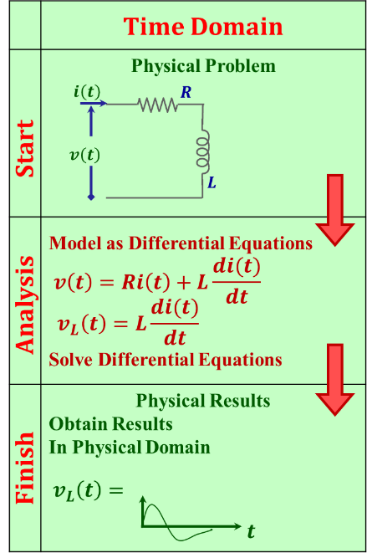
Figure 1.1: Demonstrates the process of performing analysis in the time domain.
Figure 1.1: Demonstrates the process of performing analysis in the time domain.
An alternate approach to working in the time domain is to convert the problem to the frequency domain early in the process and carry out the solution there and convert the solution back to the time domain at the end, see Figure 1.2.
The use of red downward arrows on the time domain side is to indicate the difficulties that this approach faces. As we said before, we can use the Laplace transform once we reach the point where we have “complicated” differential equations, however, the frequency domain approach avoids the need to develop the differential equations in the first place.
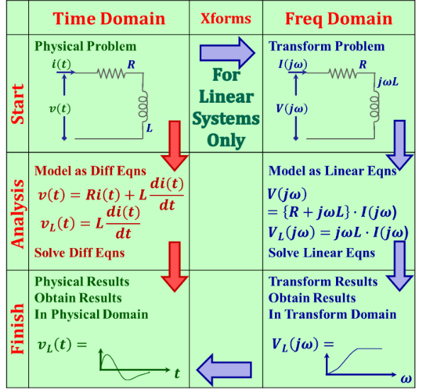
Figure 1.2
Figure 1.2
In our electrical engineering education, the frequency domain approach dominates the EE curriculum to the point that most of us have lost our relationship with the time domain altogether.
What happened was that we started out with the time domain approach and we did a few examples and simple cases there. Later on, we introduced the frequency domain and we learned how to do the whole process from the physical problem in the time domain concluding by the inverse transformation of the final results again in the time domain. Soon afterwards, we learned how to jump from the physical model into the frequency‐domain circuit model, run all our analyses and reach the results in the frequency domain and end there. We simply lose touch with the physics of the problem and the physics of the analyses. It takes additional training and experience to be able to relate the frequency domain results to the physics of the system without going back to the time domain.
Figure 1.3
Figure 1.3
In this regard, here are a couple of interesting analogies that you may find useful:
- Working in the time domain is like being awake in real life where we witness events as they occur and experience problems and issues as they happen. Suppose we encounter “this” complication that we cannot resolve. Next, we go to “sleep” and dream a solution for this problem during our sleep, and we use magical tools and reach great results to the “complicated” issue in our “dream world”. However, after we wake up, we need to be able to translate those “dream world” solutions to physical solutions that are meaningful in real life. Some would argue, the frequency domain is not a “dream world”, I argue back by asking: what do you think $"j=\sqrt{-1}"$ is? “$j$” is an imaginary quantity in an imaginary domain.
- The second analogy is that we are in a “shore” city. Our goal is to get from one part of town to another. With congested traffic and complicated routes, we decide to take the waterway that is faster and straightforward. Hence, we move from land to sea, make our way through the waterway, and when it is the right location, we move back to the land again. If we chose a waterway close to the shore, we can maintain an eye on the city’s landmarks and do not lose our orientation. We stay in touch with the city and its realities, that is. However, if we take a waterway deep in the sea, we stand a chance of losing our orientation and we will certainly lose our feel for the city and its landmarks.
It is true that with extra training and experience we can relate the “dream” to reality or stay on the course without monitoring the city’s landmarks. Therefore, we can always come up with physical interpretations to all the frequency domain terms, procedures, and conclusions. For example, “$j$” is a 90 degrees phase shift, resonance at certain frequency means energy bouncing back and forth between storage in electric and magnetic forms, and a product of transfer functions corresponds to the impulse response of their cascade, etc. However, it is always a plus to stay in touch with the physics of the problems. This yields deeper understanding and stronger comprehension, and often leads to new discoveries.
States and Languages:
Now, which domain should we use, and how to decide? Here is another analogy (please refer to Figure 1.4). It is typical for people living in the state of England to communicate in English, while residents of France do so in French. However, it is possible in some cases, although untypical, that people in France would communicate in English, and those in England do so in French.
| State | ||
| Language | England | France |
| English | 1 | 2 |
| French | 2 | 1 |
| 1 Conventional 2 Unconventional but valid |
||
| State | ||
| Language | Transient | Steady State |
| Time Domain | 1 | 2 |
| Frequency Domain | 1 | 2 |
Figure 1.4
Likewise, transient state and steady state are states while Time Domain and Frequency Domain analyses are forms of communication or expression languages. Hence, it is typical to do transient analysis in the time domain and steady state (harmonic) analysis in the frequency domain. However, for certain special cases, we do the opposite.
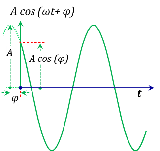
Figure 1.5
Figure 1.5
Phasors and Frequency Domain (Harmonic) Analysis:
It is known that harmonic excitation of linear systems yields harmonic solutions of the same frequency as that of the excitation. In such case, all signals throughout the entire system (circuit) will be of the same frequency with differing magnitudes and phases.
The general form of a typical time harmonic signal in the time domain would be $\ A\ cos\ (\omega{}t+\varphi{})$, see Figure 1.5. In the frequency domain, we represent this time varying function by a “phasor” of magnitude $A$ and a phase angle $\ \varphi{}$ rotating at an angular speed $\ \omega{}$, see Figure 1.6.
$ \bar{A} = A \angle (\omega t + \varphi) $
(1.1)
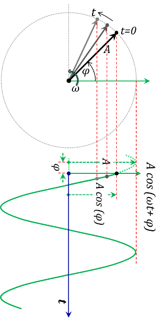
Figure 1.6
Figure 1.6
Using analogies to the mechanical harmonic motion and the conversion of rotational motion into a reciprocating one, the relationship between the time domain representation (the cosine function) and the phasor representation is better demonstrated in Figure 1.6. In this figure, the time domain waveform is presented as the projection of the rotating phasor on the “horizontal” axis.
With this graphical phasor representation of the harmonic signal, an intriguing question arises. Why do we view only the “horizontal” projection of the phasor diagram? What can we make out of its “vertical” projection? The answer is that the vertical projection is in fact complementary to the horizontal projection and it coexists whether we pay attention to it or not. In other words, its inclusion in the picture does not add any knew parameters to the physics of the problem.
The question now is, if we were to include this complementary term in our mathematical analysis without altering the nature of the original harmonic signal term or having the two terms mix or interfere, or affect the accuracy of the analysis or alter the final result, would that be unacceptable? The logical answer is no. As will be demonstrated later in this section, this inclusion (in the proper manner) greatly facilitates the mathematical analysis.
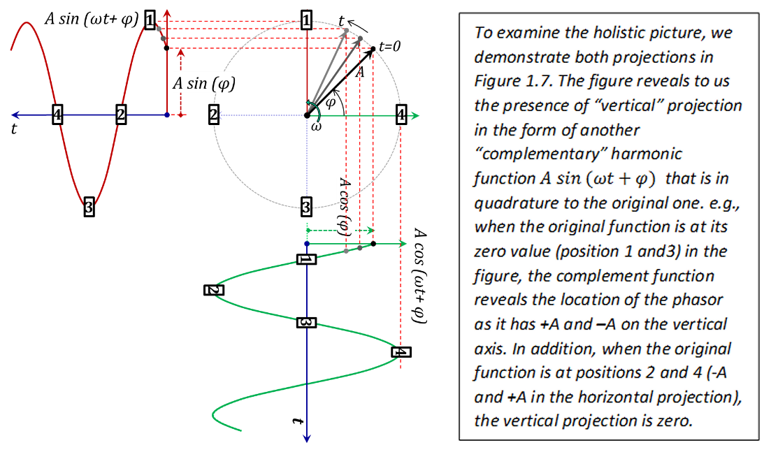
Figure 1.5
Figure 1.7
Referring to the Addendum at the end of this chapter, we can pack the harmonic function and its complement, into a one‐pack term to express the harmonic phasor in all relevant mathematical analyses. This term is known as the complex phasor and can be expressed as the sum of both real and imaginary components. Its expression in the complex domain is of the form
$ \overline{A}=\left[A\cos{\left(\omega{}t+\varphi{}\right)}\right]+j\ \left[A\sin{\left(\omega{}t+\varphi{}\right)}\right] $
(1.2)
This phasor can also be expressed in it magnitude and phase angle format:
\[ \overline{A}=A\angle{}\left(\varphi{}\right) \]
Furthermore, the use the Euler formula provides a convenient mathematical format that greatly facilitates relevant mathematical operations and procedures:
$ \overline{A}\left[=A\angle{}\left(\varphi{}\right)\right]=A\cdot e^{j(\varphi{})}=A\ cos\ \left(\varphi{}\right)+j\cdot A\ sin\ \left(\varphi{}\right)\ %eq3 $
(1.3)
Consequently, to recover the time domain expression of the harmonic signal, all needed is to extract the real part of the phasor "pack", hence:
$
C\ cos\ \left(\gamma{}\right)=Re\ \left\{C\cdot e^{j(\gamma{})}\right\}
$
(1.4)
Now, it is relevant to emphasize that:
- as we use the “pack” phasor term expression in our analysis, our goal is to recover the physically acceptable result by simply eliminating the imaginary term.
- the use of Euler’s formula offers the great convenience of dealing with exponentials in contrast with potentially complicated trigonometric identities.
To demonstrate the convenience of using Euler’s exponential form for phasor expressions, let us review some of the fundamental mathematical operations in this format:
Addition and Subtraction:- Time Domain Representation: \[ A\ cos\ \left(\omega{}t+{\varphi{}}_A\right)\pm{}B\ cos\ \left(\omega{}t+{\varphi{}}_B\right)=C\ cos\ \left(\omega{}t+{\varphi{}}_C\right) \]
- Phasor Representation: \[ \left[A\cdot e^{j(\omega{}t+{\varphi{}}_A)}\right]\pm{}\left[B\cdot e^{j(\omega{}t+{\varphi{}}_B)}\right]=\left[C\cdot e^{j(\omega{}t+{\varphi{}}_C)}\right] \]
- Recovering the Time Domain Representation: \begin{equation*} \begin{split} Re[C \cdot e^{j\omega t+\varphi_C}] &= Re \lbrace [A \cdot e^{j(\omega t + \varphi_A)}] \pm [B \cdot e^{j(\omega t + \varphi_B)}] \rbrace\\ &=Re [A \cdot e^{j(\omega t + \varphi_A)}] \pm Re [B \cdot e^{j(\omega t + \varphi_B)}]\\ &= A cos(\omega t + \varphi_A) \pm B cos(\omega t + \varphi_B)\\ \end{split} \end{equation*}
- Time Domain Representation: \[ a\cdot A\ cos\ \left(\omega{}t+{\varphi{}}_A\right)=C\ cos\ \left(\omega{}t+{\varphi{}}_C\right) \]
- Phasor Representation:\[ \left\{a\cdot \left[A\cdot e^{j(\omega{}t+{\varphi{}}_A)}\right]\right\}=\left[\left\{a\cdot A\right\}\cdot e^{j(\omega{}t+{\varphi{}}_A)}\right] \]
- Recovering the Time Domain Representation: \[ Re\left\{a\cdot \left[A\cdot e^{j(\omega{}t+{\varphi{}}_A)}\right]\right\}=a\cdot Re\left[A\cdot e^{j(\omega{}t+{\varphi{}}_A)}\right]=aA\ cos\ \left(\omega{}t+{\varphi{}}_A\right) \]
- Time Domain Representation: \begin{equation*} \begin{split} \frac{d[Acos(\omega t + \varphi_A)]}{dt} &= -\omega A sin(\omega t + \varphi_A)\\ &= \omega A cos(\omega t + \varphi_A + \frac{\pi}{2}) \end{split} \end{equation*}
- Phasor Representation:
\begin{equation} \begin{split} \frac{d}{dt}[A \cdot e^{j(\omega t + \varphi_A)}] &= [j\omega A \cdot e^{j(\omega t + \varphi_A)}] &= [\omega A \cdot e^{j(\omega t + \varphi_A + \frac{\pi}{2})}]\\ \end{split} \end{equation}
(1.5)
- Recovering the Time Domain Representation:\begin{equation*} \begin{split} Re \left \lbrace \frac{d}{dt} [A \cdot e^{j\omega t + \varphi_A}] \right \rbrace &= Re\lbrace j\omega \cdot [A \ \cdot e^{j(\omega t + \varphi_A)}]\rbrace = \omega A \cdot Re[e^{j(\pi/2)}\cdot e^{j(\omega t + \varphi_A)}]\\ &= \omega A cos (\omega t + \varphi_A +\pi/2) = -\omega A sin(\omega t + \varphi_A)\\ &= \frac{d}{dt}[Acos(\omega t + \varphi_A)] \end{split} \end{equation*}
- Time Domain Representation: \[ P_{av}=av\left\{V_{pk}\ cos\ \left(\omega{}t+{\varphi{}}_V\right)\cdot I_{pk}\ cos\ \left(\omega{}t+{\varphi{}}_I\right)\right\}=(1/2)V_{pk}I_{pk}cos({\varphi{}}_V-{\varphi{}}_I) \]
- Phasor Representation:
$P_{av}=Re\left\{\left[\left(V_{pk}/\sqrt{2}\right)\cdot e^{j(\omega{}t+{\varphi{}}_V)}\right]\cdot {\left[\left(I_{pk}/\sqrt{2}\right)\cdot e^{j(\omega{}t+{\varphi{}}_I)}\right]}^*\right\} $
(1.6)
- Recovering the Time Domain Representation: \begin{equation*} \begin{split} P_{av}&=Re \lbrace [(V_{pk}/\sqrt{2})\cdot e^{j(\omega t +\varphi_V)}]\cdot [(I_{pk}/\sqrt{2})\cdot e^{j(\omega t +\varphi_I)}]^* \rbrace\\ &=Re\lbrace (1/2) \cdot [V_{pk} \cdot I_{pk} \cdot e^{j(\varphi_V-\varphi_I)}]\rbrace\\ &=(1/2)V_{pk}I_{pk}cos(\varphi_V-\varphi_I)\\ \end{split} \end{equation*}
Use of Phasors in Circuit Analysis (in the Frequency Domain)
Performing circuit analysis using phasor “packs” is typically known as Frequency domain analysis. This terminology reflects the fact that the analysis is performed for one frequency at a time (single harmonic). The Euler expression of the phasor displays only the phasor’s magnitude and phase and not its frequency; however, the phasor frequency must be defined and is an integral part of the analysis and its solution.
Demonstration of Circuit Analysis in the Frequency Domain:
Starting with the time domain form:To demonstrate the above‐discussed concepts, let us consider a simple R‐L circuit excited by a harmonic voltage source, Figure 1.8. The desired results are to evaluate the current in the loop, the voltages across the resistor and inductor, as well as the power dissipated in the resistor.
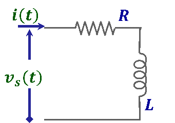
Figure 1.8
Figure 1.8
We assume that the voltage source is a harmonic source with an amplitude of V$_{s}$, radial frequency $\omega{}$, and a phase angle of $\varphi{}$$_{vs}$ at the instant t=0 (the time reference for this analysis). Hence, we can express v$_{s}$(t) in the time domain as:
$ v_s\left(t\right)=V_s\cos{\left(\omega{}t+{\varphi{}}_{vs}\right)} $
(1.7)
Now, we write KVL around the only loop in the circuit, thus:
$v_s\left(t\right)=R\cdot i_{Loop}\left(t\right)+L\cdot \frac{di_{Loop}(t)}{dt}$ where ${{\text{v}}_{\text{L}}}\left( \text{t} \right)=\text{L}\cdot \frac{\text{d}{{\text{i}}_{\text{Loop}}}\left( \text{t} \right)}{\text{dt}}$
(1.8)
Next, we write the time domain expression for the loop current in the form:
$i_{Loop}\left(t\right)=I_{Loop}\cos{\left(\omega{}t+{\varphi{}}_i\right)}$
(1.9)
where $I_{Loop}$ is the peak amplitude and $\varphi{}$$_{i}$ is the corresponding phase.
Now, the KVL expression (1.8) in the time domain takes on the form:
\begin{equation} \begin{split} {\left\{v_s\left(t\right)\right\}=V}_s\cos{\left(\omega{}t+{\varphi{}}_{vs}\right)} &=R\ I_{Loop}\cos{\left(\omega{}t+{\varphi{}}_i\right)}+L\frac{d\left[{\ I}_{Loop}\ cos\ \left(\omega{}t+{\varphi{}}_i\right)\right]}{dt}\\ &=R\ I_{Loop}\cos{\left(\omega{}t+{\varphi{}}_i\right)}-\omega{}L{\ I}_{Loop}\sin{\left(\omega{}t+{\varphi{}}_i\right)}\\ &=R\ I_{Loop}\ cos\ \left(\omega{}t+{\varphi{}}_i\right)+\omega{}L{\ I}_{Loop}\ cos\ \left(\omega{}t+{\varphi{}}_i+\pi{}/2\right) %eq10 \end{split} \end{equation}
(1.10)
Working backward towards the phasor representation, we can replace the cos terms as the real part of the complex Euler (exponential) form:
\begin{equation*} \lbrace v_s(t) \rbrace = V_s Re[e^{j(\omega t + \varphi_{vs})}] = RI_{Loop}Re[e^{j(\omega t + \varphi_i)}]+\omega LI_{Loop}Re[e^{j(\omega t + \varphi_i + \pi/2)}] \end{equation*}
\begin{equation*} \begin{split} \lbrace v_s(t) \rbrace &= Re[V_se^{j(\omega t + \varphi_{vs})}] = Re[RI_{Loop}e^{j(\omega t + \varphi_i)}]+Re[\omega LI_{Loop} e^{j(\omega t + \varphi_i)}e^{j(\pi/2)}]\\ &= Re[RI_{Loop}e^{j(\omega t + \varphi_i)}] + Re[j\omega L I_{Loop}e^{j(\omega t + \varphi_i)}] \end{split} \end{equation*}
\begin{equation*} \lbrace v_s(t) \rbrace = Re[V_s e^{j(\omega t +\varphi_{vs})}] = Re[(R+j\omega L)I_{Loop}e^{j(\omega t + \varphi_i)}] \end{equation*}
\begin{equation*} \lbrace v_s(t) \rbrace = Re[V_s e^{j(\varphi_{vs})}e^{j(\omega t)}] = Re[(R+j\omega L)I_{Loop}e^{j(\varphi_i)}e^{j(\omega t)} ] \end{equation*}
$\lbrace v_s(t)\rbrace = Re[\bar{V_s} e^{j(\omega t)}] = Re[(R+j\omega L)\bar{I}_{Loop}e^{j(\omega t)}]$
(1.11)
Where the voltage and current phasors notations ${\overline{V}}_s\ and\ \ {\overline{I}}_{Loop}\ $are used in place of ${\ V}_s\ e^{j\left({\varphi{}}_{vs}\right)}\ and\ I_{Loop}e^{j\left({\varphi{}}_i\right)}$ respectively.
Examining equation (1.11), we recognize that it represents the real part of the complex form:
$[\bar{V}_s e^{j(\omega t)}]=[(R+j\omega L)\bar{I}_{Loop}e^{j(\omega t)}]$ , or
$\bar{V}_s = (R+j\omega L)\bar{I}_{Loop}$
(1.12)
(1.13)
which is the phasor form of the KVL equation for the circuit represented in the frequency domain.
Now, using (1.12), we can solve for ${\overline{I}}_{Loop}$ as
$[\bar{I}_{Loop}]=\frac{[\bar{V}_s]}{(R+j\omega L)}$
(1.14)
From which the time domain expression for $i_{Loop}$ can be obtained through multiplying the phasor expression by $e^{j\left(\omega{}t\right)}$then extracting the real part of the product:
$\left\{i_{Loop}\left(t\right)\right\}=Re\left[{{\overline{I}}_{Loop}\ e}^{j\left(\omega{}t\right)}\right]$
(1.15)
Likewise, we can derive expressions for the time domain form of the voltage drops across the resistor and the inductor as well as the power dissipated in the resistor:
Now, let us tackle this example from the Frequency domain end. We start by converting the circuit to its Frequency domain model; voltage and currents assume their phasor formats, while circuit elements take on their impedance/admittance expressions. The result is shown in Figure 1.9.
$[\bar{V}_R] = (R)[\bar{I}_{Loop}] \xrightarrow{yields} \lbrace v_R(t) \rbrace = Re[\bar{V}_R e^{j(\omega t)}]$
(1.16)
$[\bar{V}_L] = (j\omega L)[\bar{I}_{Loop}] \xrightarrow{yields} \lbrace v_L(t) \rbrace = Re[\bar{V}_L e^{j(\omega t)}]$
(1.17)
$P_R = Re \lbrace (1/2) \cdot [\bar{V}_R] [\bar{I}^*_{Loop}] \rbrace$
(1.18)
The short version for carrying out this analysis starts by converting the circuit in Figure 1.8 to its frequency domain model, Figure 1.9.
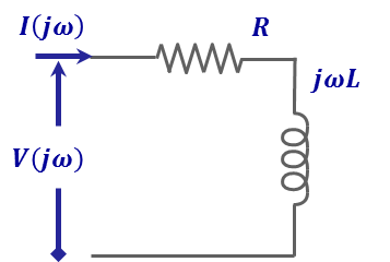
Figure 1.9
Figure 1.9
Next, we write KVL for the loop in phasor terms:
$\left[{\overline{V}}_s\right]=\left(R+j\omega{}L\right)\ \left[{\overline{I}}_{Loop}\right]$
(1.19)
Which we typically write in the frequency domain form
\[ V_s\left(j\omega{}\right)=\left\{R+j\omega{}L\right\}\cdot I_{Loop\ }\left(j\omega{}\right), \] where ${V_R\left(j\omega{}\right)=R\cdot I_{Loop\ }\left(j\omega{}\right)\ \ and\ \ V}_L\left(j\omega{}\right)=j\omega{}L\cdot I_{Loop\ }(j\omega{}$)
Hence, we continue the solution as before:
\[ I_{Loop\ }(j\omega{})=\frac{V_s\left(j\omega{}\right)}{\left(R+j\omega{}L\right)}\ \ \stackrel{yields}{\rightarrow{}}\ \ \left\{i_{Loop}\left(t\right)\right\}=Re\left[{I_{Loop\ }(j\omega{})\ e}^{j\left(\omega{}t\right)}\right] \]
\[ V_R\left(j\omega{}\right)=\left(R\right)\ I_{Loop\ }(j\omega{})\ \ \stackrel{yields}{\rightarrow{}}\ \ \left\{v_R\left(t\right)\right\}=Re\left[{V_R\left(j\omega{}\right)\ e}^{j\left(\omega{}t\right)}\right] \]
\[ V_L\left(j\omega{}\right)=\left(j\omega{}L\right){\ I}_{Loop\ }(j\omega{})\ \ \stackrel{yields}{\rightarrow{}}\ \ \left\{v_L\left(t\right)\right\}=Re\left[{V_L\left(j\omega{}\right)\ e}^{j\left(\omega{}t\right)}\right] \]
\[ P_R=Re\left\{\left(1/2\right)\cdot \left[V_R\left(j\omega{}\right)\ \right]\left[{I_{Loop}^*}_{\ }(j\omega{})\right]\right\} \]
Which yields identical results to those obtained earlier in equations (1.14) - (1.18)
The Frequency Domain and the Laplace Transform:
In this section, we briefly remind the reader of the Laplace transform and how it relates to the Frequency Domain. As you recall from other Signals and Systems studies, the Laplace transform allows us to convert time domain expressions (signals as well as system responses) into the Laplace or s-Domain. The Laplace transform expression of a time domain function $f(t)$ is given by:
$F(s)=\int_0^\infty f(t)e^{-st}dt$
(1.20)
The obtained transform $F(s)$ is expressed in the complex s-domain where $s = $$\sigma{}$+j$\omega{}$. This transform tool enables us to solve time domain transient problems through the conversion of complicated differential equations to much more manageable algebraic equations. The transform enables us to solve steady state harmonic analyses as well since letting the real part $\sigma{}$ = 0, the $F(s)$ converges to $F(j$$\omega{}$) which is the Frequency domain phasor expression for $f(t)$ function.
If we were to solve the same example of Figure (1.9) in the s-domain, we would replace the $j$$\omega{}$ in the KVL loop equation (1.19) by s. Hence
$V_s(s)=(R+sL)I_{Loop}(s)$
(1.21)
Addendum
The Mystery of $j$ and Imaginary Numbers
Suppose we package both horizontal and vertical projection terms of the rotating phasor, the harmonic function $\left[A\cos{\left(\omega{}t+\varphi{}\right)}\right],\ $and its complement$\ \left[A\sin{\left(\omega{}t+\varphi{}\right)}\right]$, into a one pack term, e.g. $P_{A}$. This pack term is to be used to express the phasor in all relevant mathematical analyses. Hence, the $P_{A}$ term needs to take the simple form of a linear mix of the harmonic function and its complement to facilitate the separation process when needed.
Hence, we write:
${{\text{P}}_{\text{A}}}=\left[ \text{A}\cos \left( \text{ }\!\!\omega\!\!\text{ t}+\text{ }\!\!\varphi\!\!\text{ } \right) \right]+\text{q }\!\!~\!\!\text{ }\left[ \text{A}\sin \left( \text{ }\!\!\omega\!\!\text{ t}+\text{ }\!\!\varphi\!\!\text{ } \right) \right]$ or
$\text{ }\!\!~\!\!\text{ }\!\!~\!\!\text{ }\!\!~\!\!\text{ }{{\text{P}}_{\text{A}}}=\left[ \text{A}\cos \left( \text{ }\!\!\alpha\!\!\text{ } \right) \right]+\text{q }\!\!~\!\!\text{ }\left[ \text{A}\sin \left( \text{ }\!\!\alpha\!\!\text{ } \right) \right]\text{ }\!\!~\!\!\text{ }\!\!~\!\!\text{ }\!\!~\!\!\text{ }$ for short
(1.22)
(1.23)
where $q$ is the mixing coefficient.
Now, let us assume another phasor B in the same analysis that would interact mathematically with the phasor A. In a similar way, we would express its harmonic function and corresponding complement into a one pack term $P_{B}$, where
$P_B=\left[B\cos{\left(\beta{}\right)}\right]+q\ \left[B\sin{\left(\beta{}\right)}\right]$
(1.24)
Now, we examine the results obtained by putting the packed terms $P_{A}$ and $P_{B}$ through different mathematical procedures that are typically required in the analysis of harmonic signals. The goal is to decide if the obtained results for the packed terms maintain the separability that allows us to retrieve the proper harmonic analysis results. We will demonstrate here some of these typical mathematical procedures, namely scaling (multiply or divide by a scalar), addition/subtraction, multiplication, and differentiation.
Scaling:Let us start by the scaling operation by considering the pack $P_{A}$ scaled by the scalar "$a$", hence
\[ {a\cdot P}_A=a\cdot \left\{\left[A\cos{\left(\alpha{}\right)}\right]+q\ \left[A\sin{\left(\alpha{}\right)}\right]\right\}=\left\{\left[a\cdot A\cos{\left(\alpha{}\right)}\right]+q\ \left[a\cdot A\sin{\left(\alpha{}\right)}\right]\right\} \]
Thus concluding that the scaling operation did not affect the separability of both the cosine and sine terms.
Addition/Subtraction:The sum $a.P_A+{b.P}_B$ yields
\begin{equation*} \begin{split} a \cdot P_A + b\cdot P_B &= \lbrace [a \cdot A \cos(\alpha)]+q[a \cdot \sin(\alpha)]\rbrace \pm \lbrace [b \cdot B\cos(\beta)] + q[b \cdot B\sin(\beta)] \rbrace\\ &= \lbrace [a\cdot A \cdot \cos(\alpha) \pm b \cdot B\cdot \cos(\beta)] + q\cdot [a \cdot A \cdot \sin(\alpha) \pm b \cdot B \cdot \sin(\beta)] \rbrace \end{split} \end{equation*}
It is clear that the sum of the cosine terms is separable from that of the sine terms, which makes our packaging scheme plausible so far.
Differentiation:
This time, we will check the differentiation operation before multiplication for a good reason. As it turned out, the multiplication operation is the one that will define the constraints on the mixing coefficient q. Hence, we will check multiplication last.
The derivative of the harmonic signal $A\cos \left( \omega t+\varphi \right)$ results into another harmonic signal $D\cos \left( \omega t+\delta \right)$ where
$\text{D}\cos \left( \text{ }\!\!\omega\!\!\text{ t}+\text{ }\!\!\delta\!\!\text{ } \right)=\frac{\partial \left[ \text{A}\cos \left( \text{ }\!\!\omega\!\!\text{ t}+\text{ }\!\!\varphi\!\!\text{ } \right) \right]}{\partial \text{t}}=-\text{ }\!\!\omega\!\!\text{ A}\sin \left( \text{ }\!\!\omega\!\!\text{ t}+\text{ }\!\!\varphi\!\!\text{ } \right)=\text{ }\!\!~\!\!\text{ }\!\!\omega\!\!\text{ A}\cos \left( \text{ }\!\!\omega\!\!\text{ t}+\text{ }\!\!\varphi\!\!\text{ }+\text{ }\!\!\pi\!\!\text{ }/2 \right)$
(1.25)
which means that $D=\omega A~$ and $\delta =\varphi +\pi /2$.
Now, we apply the derivative to the pack ${{P}_{A}}=\left\{ \left[ A\cos \left( \omega t+\varphi \right) \right]+q\text{ }\!\!~\!\!\text{ }\left[ A\sin \left( \omega t+\varphi \right) \right] \right\}$ and expect the resulting pack of the form
${{P}_{D}}=\left\{ \left[ D\cos \left( \omega t+\delta \right) \right]+q\text{ }\!\!~\!\!\text{ }\left[ D\sin \left( \omega t+\delta \right) \right] \right\}$
${{\text{P}}_{\text{D}}}=\frac{\partial \left\{ {{\text{P}}_{\text{A}}} \right\}}{\partial \text{t}}=\frac{\partial \left\{ \left[ \text{A}\cos \left( \text{ }\!\!\omega\!\!\text{ t}+\text{ }\!\!\varphi\!\!\text{ } \right) \right]+\text{q }\!\!~\!\!\text{ }\left[ \text{A}\sin \left( \text{ }\!\!\omega\!\!\text{ t}+\text{ }\!\!\varphi\!\!\text{ } \right) \right] \right\}}{\partial \text{t}}$$=\left[ -\text{ }\!\!\omega\!\!\text{ A}\sin \left( \text{ }\!\!\omega\!\!\text{ t}+\text{ }\!\!\varphi\!\!\text{ } \right) \right]+\text{q }\!\!~\!\!\text{ }\left[ \text{ }\!\!\omega\!\!\text{ A}\cos \left( \text{ }\!\!\omega\!\!\text{ t}+\text{ }\!\!\varphi\!\!\text{ } \right) \right]$
(1.26)
Comparing the results (1.25) and (1.26), we can conclude that differentiation of the pack form maintains the separability of the two terms.
Recognizing that the product of two phasors is supposed to yield a product phasor whose magnitude is the product of the two multipliers magnitudes and its phase is the sum of the two phasors phases. Using the notation:
\[ \overline{A}=A\angle{}\alpha{}\ ,\ \ \overline{B}=B\angle{}\beta{}\ ,\ \ and\ \ \ \ \ \ \ \ \overline{C}=C\angle{}\gamma{}\ \ \]
Then, the product $\overline{C}=\overline{A}\cdot \overline{B},is\ defined\ as\ \ \ \ \ C=A\cdot B,\ \ and\ \ \ \ \ \ \gamma{}=\alpha{}+\beta{}$
And the corresponding time domain form for $\overline{C}$ is
\[ C\cdot cos \left(\gamma{}\right)=A\cdot B\cdot cos \left(\alpha{}+\beta{}\right) \]
Hence
\[ P_C=\left\{A\cdot B\cdot cos \left(\alpha{}+\beta{}\right)+q\cdot A\cdot B\cdot sin \left(\alpha{}+\beta{}\right)\right\} \]
$P_C=\left\{A\cdot B\cdot \left[cos \left(\alpha{}\right)\cdot cos \left(\beta{}\right)-sin \left(\alpha{}\right)\cdot sin \left(\beta{}\right)\right]+q\cdot A\cdot B\cdot sin \left(\alpha{}+\beta{}\right)\right\}$
(1.27)
Now, multiplication of the two packs $P_A\ and\ P_B$ is put through to yield$\ P_C$, hence
\begin{equation*} \begin{split} P_c &= P_A\cdot P_B = \lbrace A \cdot \cos(\alpha) + q\cdot A \cdot \sin(\alpha) \rbrace \cdot \lbrace B \cdot \cos(\beta) + q \cdot B \cdot \sin(\beta) \rbrace\\ &= \lbrace A \cdot B \cdot \cos(\alpha) \cos(\beta) + q^2 \cdot A \cdot B \cdot \sin(\alpha)\cdot \sin(\beta) + 2 \cdot q \cdot A \cdot B \cdot [\sin(\alpha) \cdot \cos(\beta) + \cos(\alpha) \cdot \sin(\beta)]\rbrace \end{split} \end{equation*}
$P_C=\left\{A\cdot B\cdot \left[cos \left(\alpha{}\right)\cdot cos \left(\beta{}\right)+q^2\cdot sin \left(\alpha{}\right)\cdot sin \left(\beta{}\right)\right]+q\cdot A\cdot B\cdot sin \left(\alpha{}+\beta{}\right)\right\}$
(1.28)
For the two results 1.27 and 1.28 to agree, the quantity $q^{2}$ must equal -1, and hence $q$ should equal to the square root of "-1". Which is not a physical quantity, however, examining $q$ and $q^{2}$ in the light of phasor expressions, we recognize
$\bar{q^2} = 1 \angle \pi \quad \text{and} \quad \bar{q}=1 \angle (\pi/2)$
(1.29)
This $\overline{q}$ is what we customarily refer to as the imaginary term "$j$", (also termed as "$i$" in the literature).
$\bar{j^2} = 1 \angle \pi \quad \text{and} \quad \bar{j}=1 \angle (\pi/2)$
(1.30)
The naming of the "complementary" $q$ (now $j$) term as "imaginary" is befitting since the square root of "-1" is not physical or "real", and hence "imaginary". We also recognize that in our harmonic analysis, the original harmonic term is the one that physically exist and that the complementary term does not. True, we packed this complementary imaginary term in our analysis for mathematical convenience, but at the end of our analysis, only the physical signal is what matters and what results.
Consequently, as we use pack term expressions, e.g. $P_A=\left[A\cos{\left(\alpha{}\right)}\right]+j\ \left[A\sin{\left(\alpha{}\right)}\right],\ etc. $in our analysis, our goal is to recover the physically acceptable term for the analysis result by simply eliminating the imaginary term, hence
\[ C\ cos\ \left(\gamma{}\right)=Re\ \left\{C\ cos\ \left(\gamma{}\right)+j\ C\ sin\ \left(\gamma{}\right)\right\},\ where\ Re\ is\ short\ for\ "Real\ part\ of" \]
With the presence of both the real and imaginary components in the resulting phasor expressions, we find ourselves working in what we refer to as the complex domain.
At this point, it is relevant to state that the packing formula that we proposed earlier to combine the original "real" harmonic signal and the "imaginary" complementary term is in harmony with the Euler formula:
\[ \overline{C}\left[=C\angle{}\left(\gamma{}\right)\right]=C\cdot e^{j(\gamma{})}=C\ cos\ \left(\gamma{}\right)+j\cdot C\ sin\ \left(\gamma{}\right)\ \]
And hence,
\[ C\ cos\ \left(\gamma{}\right)=Re\ \left\{C\cdot e^{j(\gamma{})}\right\} \]
The use of the exponent form of the Euler's formula offers the great convenience of dealing with exponents in contrast with dealing with potentially complicated trigonometric identities.
It is relevant to state that the imaginary quantity $j$, equation (1.28), represent the packing factor of the "quadrature" complementary term. "$j$" as a phasor represent a unity magnitude and a $\pi{}$/2 phase (90$^\circ{}$ CCW rotation):
$j = 1 \cdot e^{\frac{j \pi}{2}} \quad \text{and} \quad j^2 = 1 \cdot e ^{2\frac{j\pi}{2}}=1 \cdot e^{j\pi}=-1$
(1.31)
And hence the famous identity
$j = \sqrt{-1}$
(1.32)
Finally, Figure 1.10 is a graphical demonstration of the concepts discussed above through expressing a phasor magnitude of "1" with different phase angles.
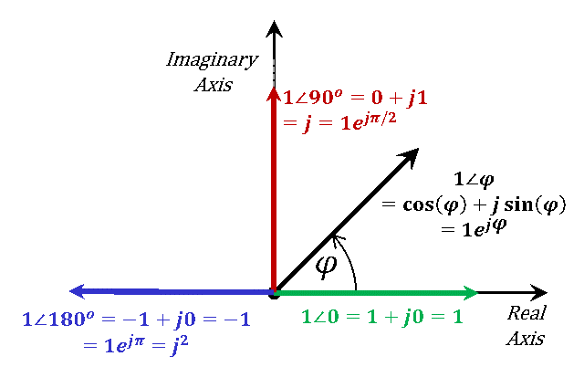
Figure 1.10
Figure 1.10
- Explain the following terms:
- Transient Analysis
- Harmonic Analysis
- Linear System
- Transient State / Steady State
- Time Domain and Frequency Domain
- Phasors
Return to Lesson
Return to Video
Examples I.1
- For the circuit of Figure 1.8, assume a source excitation of 2 Volts (rms) and a frequency of 1 $MHz$. If $R$=50 $Ohms$ and $L$= 10 $µH$, find:
- Current phasor in the loop and the Voltage phasors for both $R$ and $L$
- Time domain expressions for the obtained currents and voltages
- Repeat Example 1 for a source of the form 2u(t) Volts
Return to Lesson
Return to Video
Problems I.1
- Redo Example 1 above while adding a capacitor of 5 $nF$.
- Repeat Problem 1 for a source of the form 2u(t) Volts