1. Read the lecture (displayed below) [30-60 minutes]
2. Watch the video    [17:24 minutes]
3. Do the exercises  [~30 minutes]

Total time = [~2:00 hours]

In this lecture, we continue to further our exploration of the physics of the multiple reflections/standing waves in mismatched TL networks. Last lecture, we carried the analysis of the bounce diagram in the frequency domain.  This lecture, we will learn about the time domain version of the bounce diagram.

Again, we will consider the simple case of impedance mismatches at both the source and load ends; hence, for which multiple wave reflections occur on the line with waves bouncing back and forth between its mismatched ends.  (Same case demonstrated earlier in Figure 2.17)

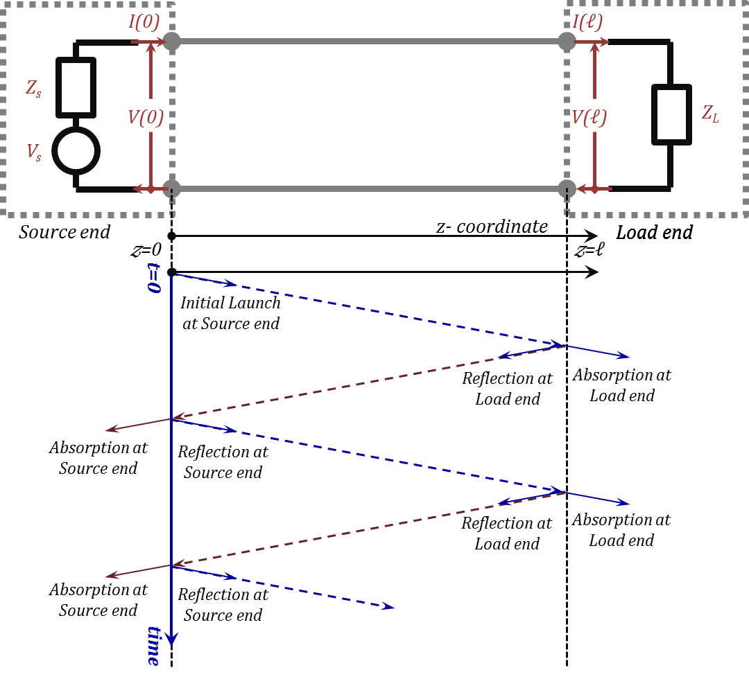
Figure 2.17

The Time Domain Bounce Diagram:

When we discussed the bounce diagram in the frequency domain, we were thinking of harmonic signals traveling back and forth on the line (in the steady state). Although we were discussing a steady state, we used a “transient” approach to construct the steady state answer.  To do the same exact thing in the time domain, i.e., use the transient approach to construct the time domain steady state answer, we will be limit the discussion to the lossless line case.  This is because the time domain analysis of lossy lines gets beyond our mathematical capabilities and our interest at this point.
 
Two main advantages to working the bounce diagram in the time domain are the following:  First, is the ability to work out transients of non-harmonic signals in simple expressions (only for lossless lines).  The second reason is related to practical application in time domain reflectometry (including practical transmission media, which are not lossless).

In time domain reflectometry, a pulse is launched in a transmission medium and its reflections are monitored.  The delay of the reflected signals is used to determine the distance (and hence location) of the medium discontinuity that caused the reflection. Meanwhile, the nature of the reflection (waveform) can be used to reveal information about the nature of the discontinuity. Practical devices are built around these concepts in many application fields.  Among those devices are RADARS that are used to locate, monitor, and identify airplanes and other flying objects.  Sonars are other devices that have applications in medical applications as well as beneath the earth explorations.  The most direct application in transmission lines is the Time Domain Refelctometer, TDR, used for cable testing and fault location.  The optical version of that is called OTDR (Optical Time Domain Refelctometer) which is used for fiber cables.

With this background in mind, we can see the importance of discussing time domain bounce-diagrams even though we will limit the analysis to lossless media. Furthermore, we will initially confine our discussion to pure resistive discontinuities including the source and load “impedances”.

Time Domain Bounce Diagram for Lossless Lines and Resistive Discontinuities:

In this discussion we will be working with the signals in their time domain form, and hence, we will be using the lower case notations, $v(z, t)$ and $i(z, t)$.  Furthermore, we will be dealing with time domain (local/instantaneous) reflection coefficients for which we will use the notation $ρ$ instead of $Γ$.  This local reflection coefficient can only be found at the discontinuities at the instant the “incident” signal reaches that discontinuity.  This concept is demonstrated in Figure 2.31.  At any instance of time, and in locations with no discontinuities, only one signal may exist.  However, at discontinuity locations, reflections off the discontinuity result in two coexisting signals, the incident signal, and its reflection.

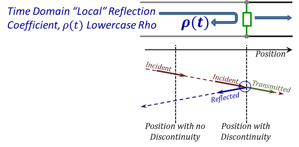
Figure 2.31

Now, consider the setup shown in Figure 2.32 with a source and load as shown.  Both source and load impedances $\left({{\text{R}}_{\text{S}}}~\text{and}~{{\text{R}}_{\text{L}}}\right)$ are purely resistive.  The transmission line connecting the two sides is assumed lossless, and hence has a pure resistive characteristic impedance ${{\text{R}}_{\text{o}}}$. Consequently, we can write the local reflection coefficients at the source and load ends of the line as:
${{\rho}_{\text{s}}}=\frac{\left[{{\text{R}}_{\text{s}}}~-~{{\text{R}}_{\text{o}}}\right]}{\left[{{\text{R}}_{\text{s}}}~+~{{\text{R}}_{\text{o}}}\right]}~~~\text{and}~~~{{\rho}_{\text{L}}}=\frac{\left[{{\text{R}}_{\text{L}}}~-~{{\text{R}}_{\text{o}}}\right]}{\left[{{\text{R}}_{\text{L}}}~+~{{\text{R}}_{\text{o}}}\right]}\tag{2.96}$

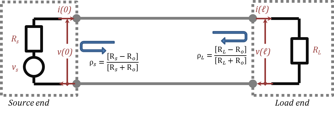
Figure 2.32

Also, the initial launch $a\left(\text{t}\right)=v\left(z=0,\text{t}=0\right)$ can be written as the voltage divider of $v_{s}(t)$ between the line’s characteristic resistance (impedance),$R_{o}$, and the source’s resistance, $R_{s}$, see Figure 2.33:
$a\left(t\right)=v\left(0\right){{|}_{t=0}}={{v}_{s}}\frac{{{R}_{o}}}{\left[{{R}_{s}}+{{R}_{o}}\right]}\tag{2.97}$ 

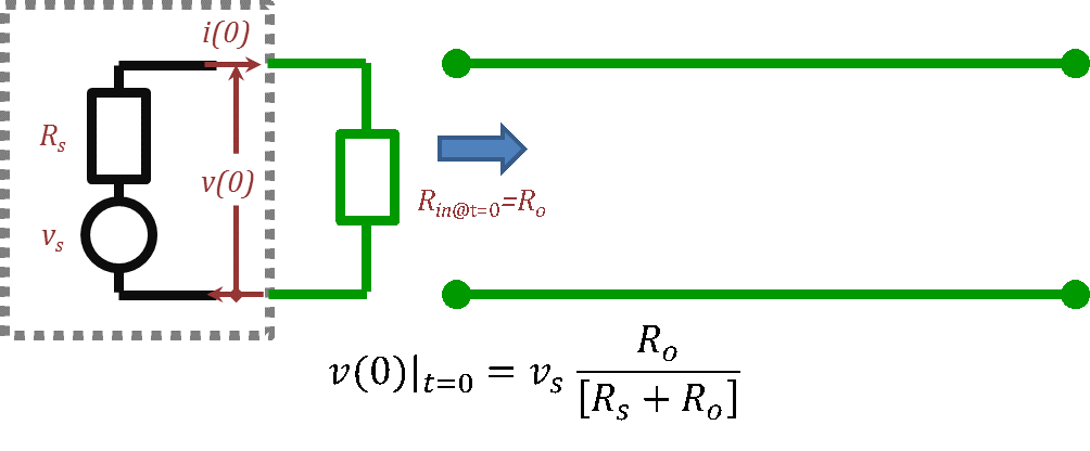
Figure 2.33

Now, we can construct the time-domain bounce diagram as we follow the signal travel (delay) and reflect (and transmit) at discontinuities (load and source resistances).  As discussed earlier, Equation (2.40), the time delay corresponding to a distance travelled is given by τ ${distance}=distance/c_{ph}$. 

Using the notation, τ = $\ell/c_{ph}$, τ$_{z }= z/c_{ph}$, and τ$_{d} = (\ell-z)/c_{ph}$, the first positive $z$ waveform is the initial launch $a(t)$ which becomes $a(t- $τ$_{z})$ after traveling a distance $z$ and $a(t- $τ) at the load. The first reflection at the load yields $[ρ_{L}].[a(t- $τ$)]$ as the first negative $z$ traveling wave.

This reflection travels back towards the source experiencing further delays to arrive at the source after a delay of $2\ell/c_{ph} = 2$τ, and hence can be written as $[ρ_{L}].[a(t- 2$τ$)]$. Reflecting from the source, a second positive $z$ travel is initiated through a reflection coefficient of $[ρ_{s}]$.
 
This signal is thus initiated as $[ρ_{s}].[ρ_{L}].[a(t-2$τ$)]$ and travels towards the load accumulating more delays. The multiple reflections go back and forth with further delays (time shift) of $distance/c_{ph}$ and amplitudes changing by the reflection coefficients multipliers $[ρ_{s}]$ and $[ρ_{L}]$. 

Now, we examine the transmission (through) waveforms that take place at the load and the source ends upon each reflection. Upon the arrival of the signal at the discontinuity, a reflection voltage develops at that discontinuity in the form of $[ρ_{s~or~L}].[incident~voltage]$.

The total voltage at that location is then equal to $[incident~voltage]+[ρ_{s~or~L}].[incident~voltage]=[1+ρ_{s~or~L}].$$[incident~voltage]$. This voltage transmits to the other side of the discontinuity whether it is the source or the load.  Consequently, the first arrival signal to the load side is of the form $[a(t-$τ$)]+[ρ_{L}].[a(t- $τ$)]= [1+ρ_{L}].[a(t- $τ$)]$ and the first arrival to the source is $[ρ_{L}].[a(t- 2$τ$)]$ $+[ρ_{s}].[ [ρ_{L}].[a(t- 2$τ$)]$ $ =[1+ρ_{s}].[ρ_{L}].[a(t- 2$τ$)]$.

The process we just discussed in the above paragraphs is demonstrated in Figure 2.34 and the resulting waveforms are summarized in Table 2.4.

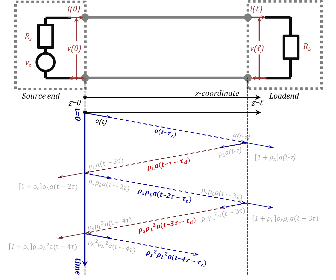
Figure 2.34

Table 2.4

 

From table 2.4, we can write expressions for the signal as a function of position and time as:
${{v}^{+}}\left(z,\text{t}\right)=a\left(\text{t}-{{\tau}_{z}}\right)+{{\rho}_{\text{s}}}~{{\rho}_{\text{L}}}~a\left(\text{t}-2\tau-{{\tau}_{z}}\right)+{{\rho}_{\text{s}}}^{2}~{{\rho}_{\text{L}}}^{2}~a\left(\text{t}-4\tau-{{\tau}_{z}}\right)+{{\rho}_{\text{s}}}^{3}~{{\rho}_{\text{L}}}^{3}~a\left(\text{t}-6\tau-{{\tau}_{z}}\right)+\cdots \tag{2.98}$
${{v}^{-}}\left(z,\text{t}\right)={{\rho}_{\text{L}}}\cdot\left\{a\left(\text{t}-\tau-{{\tau}_{\text{d}}}\right)+{{\rho}_{\text{s}}}~{{\rho}_{\text{L}}}~a\left(\text{t}-3\tau-{{\tau}_{\text{d}}}\right)+{{\rho}_{\text{s}}}^{2}~{{\rho}_{\text{L}}}^{2}~a\left(\text{t}-5\tau-{{\tau}_{\text{d}}}\right)+\cdots \right\}\tag{2.99}$
$v\left(z,\text{t}\right)={{v}^{+}}\left(z,\text{t}\right)+{{v}^{+}}\left(z,\text{t}\right)\tag{2.100}$

Time Domain Reflectometry and the Bounce Diagram:

As discussed earlier, time-domain reflectometry is a technique used for extracting information of a transmission medium by monitoring and analyzing reflections off the medium due to an incident pulse. Typical pulse shapes used in TDR devices are either a step-like waveform (a practical version of an ideal step function, $u(t)$, or an impulse (a practical version of a Dirac-delta function, $δ(t)$). In this section, we will work with the ideal waveforms for mathematical convenience.

Time-Domain Reflectometry for Ideal Step Waveform Excitations:

In this case, we assume $v_{s}(t)=V~u(t)$, where $V$ is the amplitude of the voltage step. To demonstrate the concept, let us assume the simple network of Figure 2.34 with the following parameters:
$v_{s}~=~1~u(t)~Volts$
$R_{o}~=~75~Ohms$
$R_{L}~=~125~Ohms$
$R_{s}~=~50~Ohms$
$Line~length~=~15~cm$
$Speed~of~light~in~TL~material~=~1.5~E8~m/s$

Using these parameters, we conclude that
$a(t)~=~[1~u(t)].(75)/(75+50)~=~0.6~u(t)~Volts$
$ρ_{s}~=~(50-75)/(50+75)~=~-0.2$
$ρ_{L}~=~(125-75)/(125+75)~=~0.25$
τ$~=~0.15/1.5E8~=~1~ns$

Next, we use these values to substitute in the bounce diagram of Figure 2.34 and extract the essential information from Table 2.4, namely, the TDR (time-domain reflectometry) signal (appearing at the source end, and TDT (time domain transmission) signal appearing at the load end.  The results are shown below:

Consequently, the TDR and TDT waveforms are as shown in Figure 2.35 below:

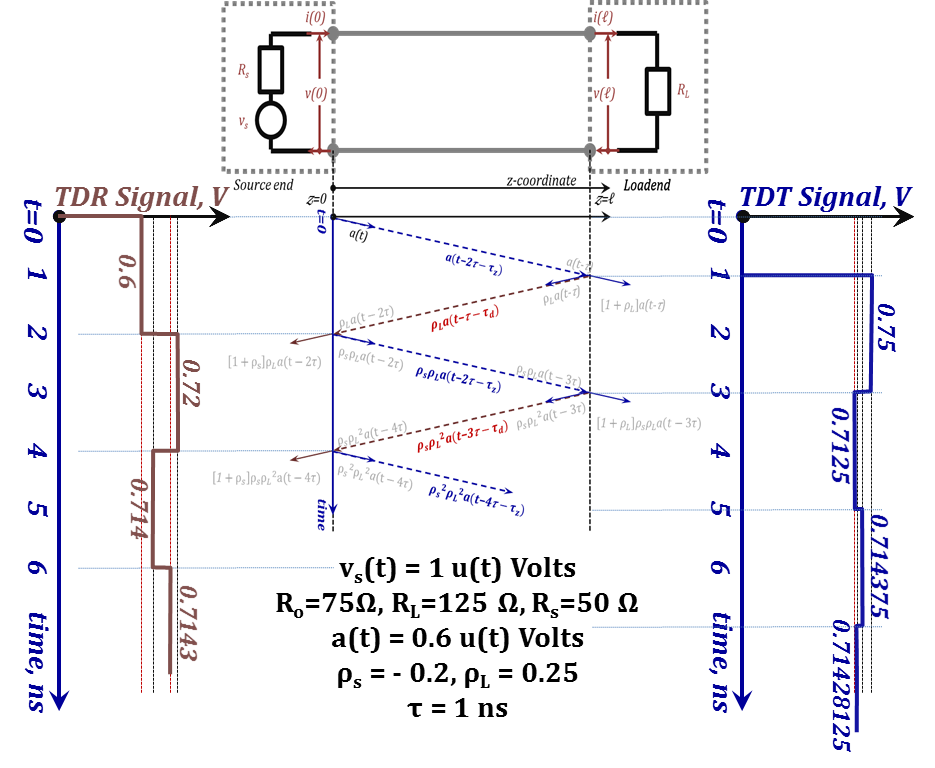
Figure 2.35

It is worth noting that both TDR and TDT signals converge to the same amplitude.  As time approaches infinity, the “final value theorem” tells us that the solution is the same as the DC solution.  For DC, the TL acts like a zero length wire, and hence both voltages at the sending and receiving ends are the same as the voltage divider between the load and source impedances:
$V_{t~=~∞~}=~V~R_{L}/(R_{s}+R_{L})~=~(1).(125)/(50+125)~=~0.7142857~V$

Time-Domain Reflectometry for Ideal Dirac-Delta Impulse Waveform Excitations:

To demonstrate, let us consider the same example we just did for the step waveform while considering $v_s~=~1~δ(t)~Volts$, hence $a(t)~=~0.6~δ(t)~Volts$ and the expressions for the TDR and TDT signals becomes:

Consequently, the TDR and TDT waveforms are as shown in the Figure 2.36  below:

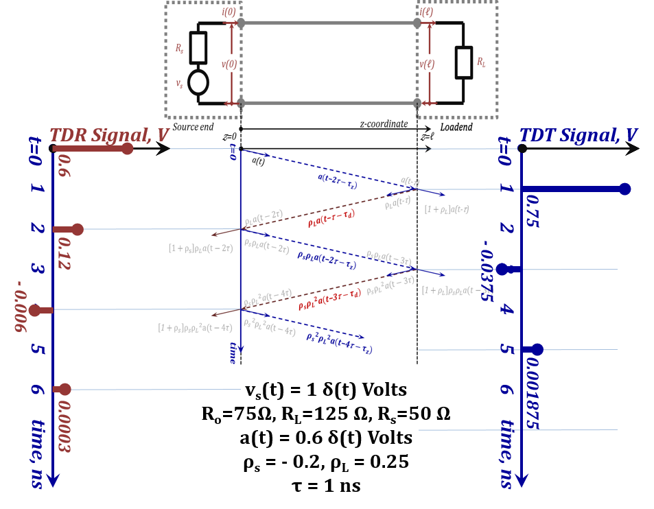
Figure 2.36

The final value in this case is a zero since $δ(t)$ vanishes when $t$ approaches infinity.

 

Video

1. Mention some applications of Time Domain Reflectometry (TDR).  
2. What is the maximum time it take a TDR device to detect a fault in a ${1~km}$ cable assuming the detection is based on observing the voltage at the pulse injection point i.e. $z=0$?  

Return to Lesson

Return to Video

1. A TDR device is used to inject a pulse, $u(t)$, into a lossless (air dielectric) cable. If the forward propagating waveform is given by $u(t-z/c)$, where $c$ is the speed of light in free space, $3\times10^8~m/s$, and the reflected waveform is given by $u(t+z/c\,-\,$τ$)$, τ$~=6~ns$. Assuming the cable has no faults, what is the load connected to the end of the cable and how long is the cable?  
2. If a fault exists half way along the cable described in the previous example, what will the voltage waveform observed at $z=0$ look like if:
   a) The fault is a short circuit.
   b) The fault is an open circuit.  

Return to Lesson

Return to Video

1. For a TDR device connected to a cable of length $1~m$ and having $Z_o=50~Ohm$ and forming a circuit similar to the one in Figure 2.34 with the TDR being the voltage source. The TDR operates by injecting a unit pulse $u(t)$ into the cable. If reflections beyond the third can be considered negligible, plot the voltage waveform at $z=0$ for a load impedance ${{Z}_{L}}=10~Ohm$. 

Return to Lesson

Return to Video

Click here to download the Instructor Guide >>