Chapter II-Lesson 4 of 10 Transmission Lines - Wave Equations
Instructions
- Read the lecture (displayed below) [30-60 minutes]
- Watch the video (13:15+17:23 minutes) [~35 minutes]
- Do the exercises [~30 minutes]
Total time = [~2:00 hours]
In previous lectures:
In the last lecture, we learned about the physical implications of the reflection coefficient $Γ(z)$ defined as the ratio between the $–z$ and $+z$ waves. We also learned about the driving point impedance $Z(z)$ and its relationship to $Γ(z)$.
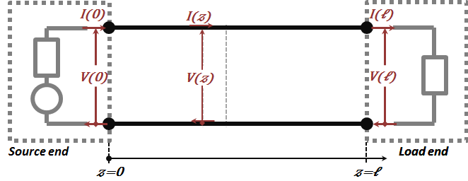
Figure 2.6

Figure 2.6
|
$\Gamma\!\!\text{ }\left( z \right)=\frac{{{\text{V}}^{-}}{{\text{e}}^{+\text{ }\gamma\text{ z}}}}{{{\text{V}}^{+}}{{\text{e}}^{-\text{ }\gamma ~ z}}}=\frac{{{\text{V}}^{-}}}{{{\text{V}}^{+}}}{{\text{e}}^{+2\text{ }\gamma~ z}}$ |
(2.43) |
|
$\text{V}\left( z \right)={{\text{V}}^{+}}{{\text{e}}^{-\text{ }\gamma\text{ z}}}\left[ 1+\text{ }\!\Gamma\!\text{ }\left( z \right) \right]$ |
(2.44) |
|
$\text{I}\left( z \right)=\frac{{{\text{V}}^{+}}{{\text{e}}^{-\text{ }\gamma z}}}{{\text{Z}_{\text{o}}}}\left[ 1-\text{ }\!\Gamma\!\text{ }\left( z \right) \right]$ |
(2.45) |
|
$\text{Z}\left( z \right)=\frac{\text{V}\left( z \right)}{\text{I}\left( z \right)}=\text{ }\!\!~\!\!\text{ }{{\text{Z}}_{\text{o}}}\frac{\left[ 1+\text{ }\!\Gamma\!\text{ }\left( z \right) \right]}{\left[ 1-\text{ }\!\Gamma\!\text{ }\left( z \right) \right]}$ and $\Gamma\!\!\text{ }\left( z \right)=\frac{\left[ \text{Z}\left( z \right)-{{\text{Z}}_{\text{o}}} \right]}{\left[ \text{Z}\left( z \right)+{{\text{Z}}_{\text{o}}} \right]}$ |
(2.46) |
|
$\text{Z}\left( 0 \right)=\frac{\text{V}\left( 0 \right)}{\text{I}\left( 0 \right)}=\text{ }\!\!~\!\!\text{ }{{\text{Z}}_{\text{o}}}\frac{\left[ 1+\text{ }\!\Gamma\!\text{ }\left( 0 \right) \right]}{\left[ 1-\text{ }\!\Gamma\!\text{ }\left( 0 \right) \right]}$ |
(2.47) |
|
$\text{Z}\left( \ell \right)=\frac{\text{V}\left( \ell \right)}{\text{I}\left( \ell \right)}=\left\{ {{\text{Z}}_{\text{L}}} \right\}=\text{ }\!\!~\!\!\text{ }{{\text{Z}}_{\text{o}}}\frac{\left[ 1+\text{ }\!\Gamma\!\text{ }\left( \ell \right) \right]}{\left[ 1-\text{ }\!\Gamma\!\text{ }\left( \ell \right) \right]}$ |
(2.48) |
|
${{\text{Z}}_{\text{L}}}=\text{ }\!\!~\!\!\text{ }{{\text{Z}}_{\text{o}}}\frac{\left[ 1+\text{ }\!\Gamma\!\text{ }\left( \ell \right) \right]}{\left[ 1-\text{ }\!\Gamma\!\text{ }\left( \ell \right) \right]}\Rightarrow \text{ }\!\Gamma\!\text{ }\left( \ell \right)=\text{ }\!\!~\!\!\text{ }\frac{\left[ {{\text{Z}}_{\text{L}}}-{{\text{Z}}_{\text{o}}} \right]}{\left[ {{\text{Z}}_{\text{L}}}+{{\text{Z}}_{\text{o}}} \right]}\text{ }\!\!~\!\!\text{ }$ |
(2.49) |
|
$\Gamma\!\!\text{ }\left( z \right)=\frac{{{\text{V}}^{-}}{{\text{e}}^{+\text{ }\gamma\text{ z}}}}{{{\text{V}}^{+}}{{\text{e}}^{-\text{ }\gamma\text{ z}}}}$ and $\text{ }\!\!\Gamma\!\!\text{ }\left( \ell \right)=\frac{{{\text{V}}^{-}}{{\text{e}}^{+\text{ }\gamma\text{ }\ell }}}{{{\text{V}}^{+}}{{\text{e}}^{-\text{ }\gamma\text{ }\ell }}}$ |
(2.50) |
|
$\Gamma\!\!\text{ }\left( z \right)=\text{ }\!\Gamma\!\text{ }\left( \ell \right)\cdot {{\text{e}}^{+2\text{ }\gamma\text{ }\left( \text{z}-\ell \right)}}=\text{ }\!\Gamma\!\text{ }\left( \ell \right)\cdot {{\text{e}}^{-2\text{ }\gamma\text{ }\left( \text{d} \right)}}$ |
(2.51) |
Standing Waves and Standing Wave Ratio:
In this lecture, we will discuss transmission lines standing waves, Standing Wave Ratio, and the Bounce Diagram in the Frequency Domain.
The combination of waves traveling in both directions on the same TL is likely to cause standing waves to form. To explain, let us start with the lossless line time- domain combined solution, Equation (2.34).
$v\left( z,\text{t} \right)=\left| {{\text{V}}^{+}} \right|\cos \left( \text{ }\!\omega\!\text{ t}-\text{ }\!\beta z+\text{ }\!\!\varphi\!\!\text{ }_{v}^{+} \right)+\left| {{\text{V}}^{-}} \right|\text{ }\!\!~\!\!\text{ cos}(\text{ }\!\omega\!\text{ t}+\text{ }\!\beta z+\text{ }\!\!\varphi\!\!\text{ }_{v}^{-})\tag{2.34}$
By adding and subtracting the term $\left| {{V}^{-}} \right|\cos \left( \omega t-\beta z+\varphi _{v}^{+} \right)$ in the right hand side of the equation, we obtain:
$v\left( z,\text{t} \right)=\left| {{\text{V}}^{+}} \right|\cos \left( \text{ }\!\omega\!\text{ t}-\text{ }\!\beta z+\text{ }\!\!\varphi\!\!\text{ }_{v}^{+} \right)+\left| {{\text{V}}^{-}} \right|\cos \left( \text{ }\!\omega\!\text{ t}+\text{ }\!\beta z+\text{ }\!\!\varphi\!\!\text{ }_{v}^{-} \right)$
$v\left( z,\text{t} \right)=\left\{ \left[ \left| {{\text{V}}^{+}} \right|-\left| {{\text{V}}^{-}} \right| \right]\cdot\cos \left( \text{ }\!\omega\!\text{ t}-\text{ }\!\beta z+\text{ }\!\!\varphi\!\!\text{ }_{v}^{+} \right) \right\}+\left\{ \left| {{\text{V}}^{-}} \right|\left[ \cos \left( \text{ }\!\omega\!\text{ t}-\text{ }\!\beta z+\text{ }\!\!\varphi\!\!\text{ }_{v}^{+} \right)+\cos \left( \text{ }\!\omega\!\text{ t}+\text{ }\!\beta z+\text{ }\!\!\varphi\!\!\text{ }_{v}^{-} \right) \right] \right\}$
$v\left( z,\text{t} \right)=\left\{ \left[ \left| {{\text{V}}^{+}} \right|-\left| {{\text{V}}^{-}} \right| \right]\cdot\cos \left( \text{ }\!\omega\!\text{ t}-\text{ }\!\beta z+\text{ }\!\!\varphi\!\!\text{ }_{v}^{+} \right) \right\}+\left\{ 2\left| {{\text{V}}^{-}} \right|\left[ \cos \left( \text{ }\!\omega\!\text{ t}+{{\text{ }\!\!\varphi\!\!\text{ }}_{1}} \right)\cdot \cos \left( \text{ }\!\beta z+{{\text{ }\!\!\varphi\!\!\text{ }}_{2}} \right) \right] \right\}\tag{2.61}$
Where ${{\varphi }_{1}}~and~{{\varphi }_{2}}$ replace the quantities $\frac{\varphi _{v}^{+}+\varphi _{v}^{-}}{2}~and~\frac{\varphi _{v}^{+}-\varphi _{v}^{-}}{2}$, respectively.
The first term of the resulting equation, $\left\{ \left[ \left| {{\text{V}}^{+}} \right|-\left| {{\text{V}}^{-}} \right| \right]\cdot\cos \left( \text{ }\!\omega\!\text{ t}-\text{ }\!\beta z+\text{ }\!\!\varphi\!\!\text{ }_{\text{v}}^{+} \right) \right\}$, has the same traveling form as the positive $z$ traveling wave but with a reduced amplitude of $\left[ \left| {{V}^{+}} \right|-\left| {{V}^{-}} \right| \right]$. On the other hand, the second term, $\left\{ 2\left| {{\text{V}}^{-}} \right|\left[ \cos \left( \text{ }\!\omega\!\text{ t}+{{\text{ }\!\!\varphi\!\!\text{ }}_{1}} \right)\cdot \cos \left( \text{ }\!\beta z+{{\text{ }\!\!\varphi\!\!\text{ }}_{2}} \right) \right] \right\}$ has an amplitude of $2\left| {{V}^{-}} \right|$ and describes a "standing wave" that does not travel in either direction on the line and is characterized by stationary "peaks/maxima" and "valleys/minima". This can be seen mathematically by examining the expression and recognizing that the spatial dependence term $\left[ \cos \left( \text{ }\!\beta z+{{\text{ }\!\!\varphi\!\!\text{ }}_{2}} \right) \right]$ forces the term to zero at certain $z$ locations irrespective of the time dependent term. This is demonstrated in Figure 2.13.
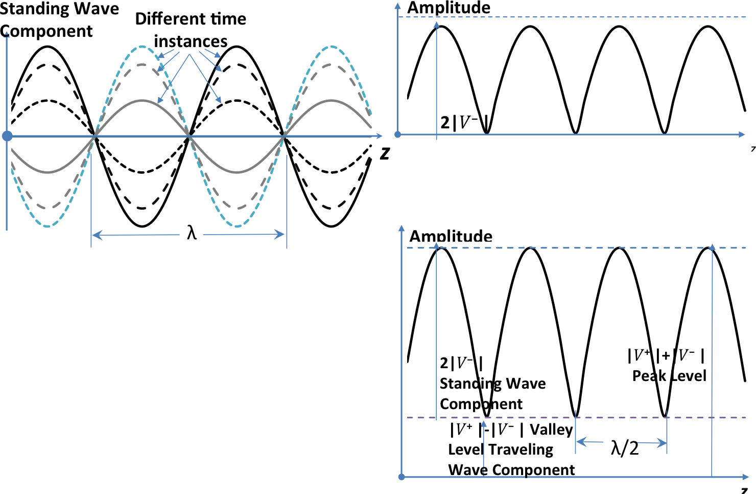
Figure 2.13
Figure 2.13
Hence, expression (2.61), as seen in the figure, is a mixture of a traveling wave component and a standing wave one. The amplitude of the standing wave component $2\left| {{V}^{-}} \right|$, is determined by the level of the reflected signal. In the absence of reflections, there will be no standing waves and we get pure traveling waves on the line. However, a $100%$ reflection where $\left| {{V}^{-}} \right|=\left| {{V}^{+}} \right|$ results in a pure "$100$%" standing waves on the TL since the traveling wave term $\left[ \left| {{\text{V}}^{+}} \right|-\left| {{\text{V}}^{-}} \right| \right]$ reduces to zero.
An important indicator of the level of standing waves in a TL network is the standing wave ratio, $\text{SWR}$, the definition for which is the ratio of the peak (max) amplitude of the signal and its valley (min) value:
$\text{SWR}=\frac{{{\left| \text{V} \right|}_{\text{max}}}}{{{\left| \text{V} \right|}_{\text{min}}}}=\frac{\left[ \left| {{\text{V}}^{+}} \right|+\left| {{\text{V}}^{-}} \right| \right]}{\left[ \left| {{\text{V}}^{+}} \right|-\left| {{\text{V}}^{-}} \right| \right]}=\frac{1+\left| \text{ }\!\Gamma\!\text{ } \right|}{1-\left| \text{ }\!\Gamma\!\text{ } \right|}\tag{2.62}$
$\text{SWR}=1$ for a pure traveling waves $(\left| \text{ }\!\Gamma\!\text{ } \right|=0)$ and $\text{SWR}=∞$ for a pure standing wave $(\left| \text{ }\!\Gamma\!\text{ } \right|=1)$.
Figure 2.14 is a graphical demonstration of the relationship between the $\text{SWR}$ and $\left| \text{ }\!\Gamma\!\text{ } \right|$.

Figure 2.14
Figure 2.14
For lossy lines, the line attenuation causes the signals to decay down the TL path, resulting in the signal forms displayed in Figure 2.15.
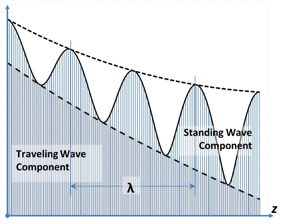
Figure 2.15
Figure 2.15
The figure shows the presence of a mixture of traveling and standing waves, just as in the lossless case. It is important to note here that since all the levels are changing, it is not possible to define a single value for the $\text{SWR}$. It is typical in such cases; to identify the location at which the $\text{SWR}$ is given, i.e., the $\text{SWR}$ of the load would be that of the nearest minimum and maximum to the TL load.
Another way of looking at the combination of the two traveling waves and their "interference" is to consider the corresponding phasor diagrams. For convenience, we will consider the case of a lossless TL only. In this case, the two phasors representing the two traveling waves are:
${{\text{V}}^{+}}{{\text{e}}^{-~j~\!\beta z}}\text{ }\!~\!\!\text{ and }\!~\!\!\text{ }{{\text{V}}^{-}}{{\text{e}}^{+~j~\!\beta z}}$
Referring to Figure 2.16, we will start with a graph of the two phasors at some location $z_{1}$ where they line up in their phase. As we move from $z_{1}$ to $z_{2}$ (where $z_{2}>z_{1}$), the phase of the $V^{+}$ phasor changes by $-\beta \left( {{z}_{2}}-{{z}_{1}} \right)$ (decreases) while the phase of the $V^{-}$ phasor changes by $+\beta \left( {{z}_{2}}-{{z}_{1}} \right)$ (increases). Similarly, we monitor the phasors' rotation as we move to ${{z}_{3}}$ and ${{z}_{4}}$. The sum of the two phasors is displayed for all four positions in part (b) of the figure, and its magnitude is plotted vs distance in part (c) of the figure. We notice that the sum exhibits the same shape as that demonstrated earlier in Figure 2.13. We also notice that the peaks (maxima) occur when the two phasors line up with equal phases. The spacing between two consecutive peaks correspond to a $180 ~degree$ rotation which is equivalent to a distance if λ$/2$.
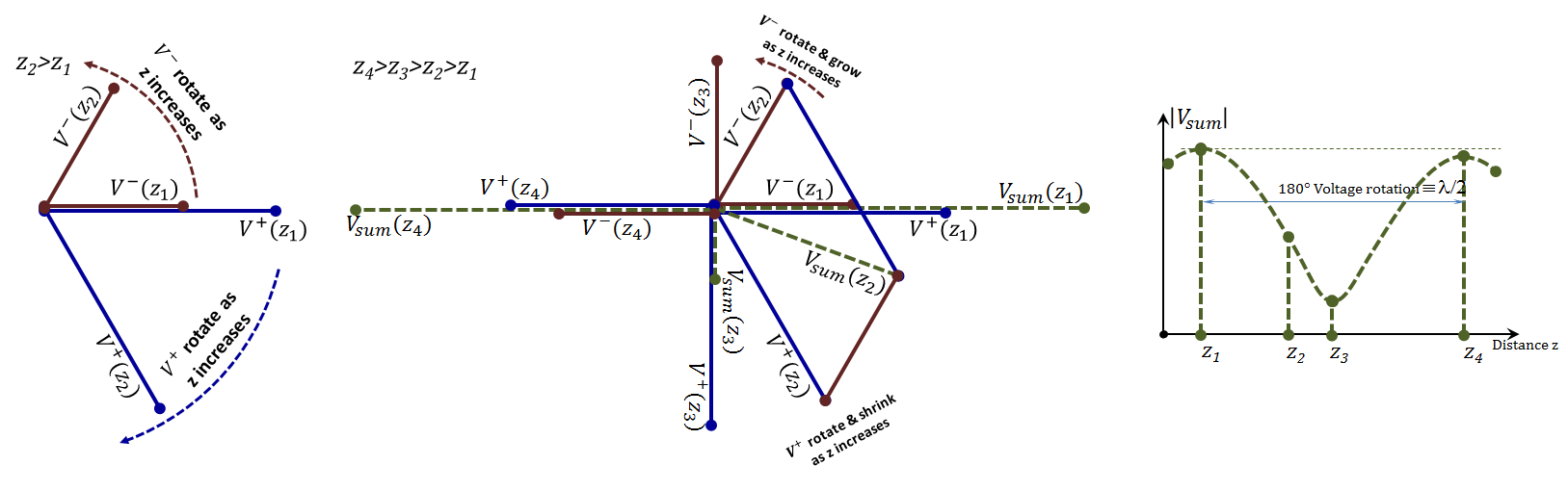
Figure 2.16
Figure 2.16
Standing Waves and the Bounce Diagram:
In this section, we further our exploration of the physics of the multiple reflections / standing waves in mismatched TL networks. In this regard, we will consider the general case of impedance mismatches at both the source and load ends; hence, we can see that multiple wave reflections will occur on the line with waves bouncing back and forth between the (generally) mismatched TL ends. Figure 2.17 depicts the TL network and the expected "bounce" diagram as a result.
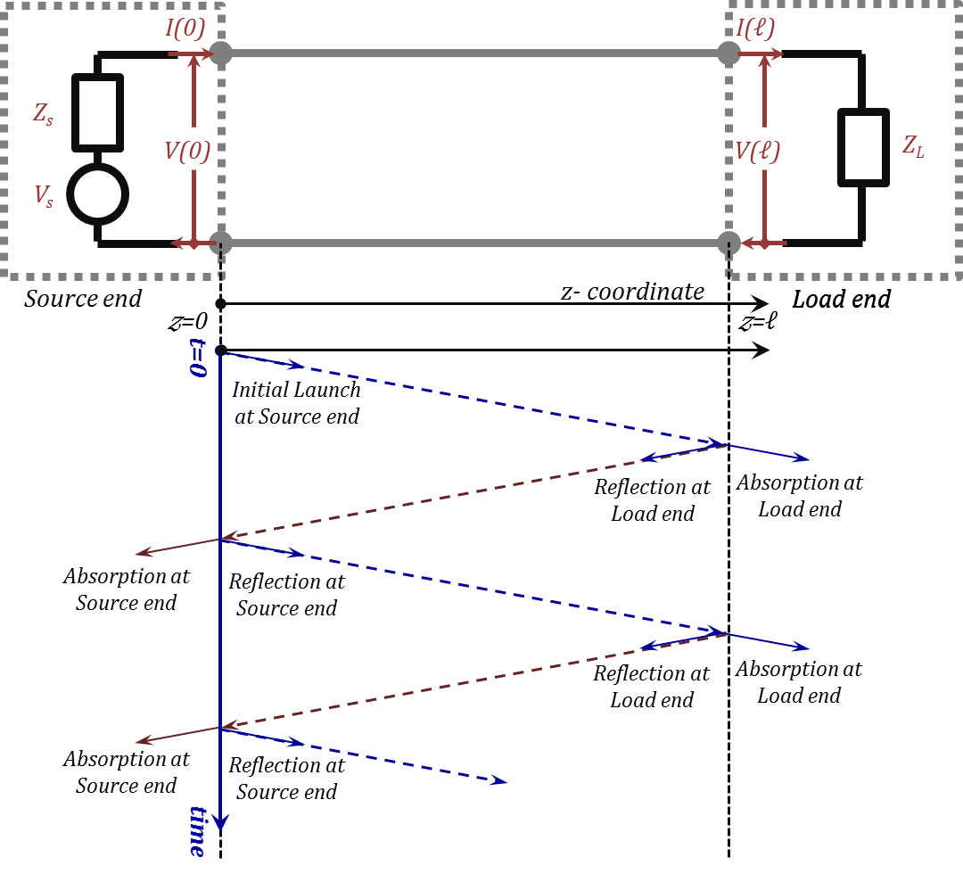
Figure 2.17
Figure 2.17
Using this bounce (reflection-transmission) diagram, let us now examine the physical meaning of the wave reflection and the corresponding reflection coefficient as defined in the frequency domain in Equation (2.50), $\Gamma\!\!\text{ }\left( z \right)=\frac{{{V}^{-}}{{e}^{+\gamma z}}}{{{V}^{+}}{{e}^{-\gamma z}}}$. We claim that the ${{V}^{-}}{{e}^{+\gamma z}}$ wave resulted from the reflections of the wave ${{V}^{+}}{{e}^{-\gamma z}}$. Meanwhile, we do not see any discontinuities at a general location $z$ that can cause reflections at that location. So, where did the ${{V}^{-}}{{e}^{+\gamma z}}$ come from? The answer lies in examining the transients build up before the steady state (harmonic) is reached.
In this regard, and based on the time-domain solution obtained earlier in Equation (2.29), a ${{v}^{+}}\left( z,t \right)$ wave, was initially launched at the sending end of the line. This wave traveled along the TL experiencing both attenuation and phase shift but no reflections until it met the first discontinuity at the load end. At the load "discontinuity", this wave suffered its first reflection triggering the backward traveling wave, ${{v}^{-}}\left( z,t \right)$. The reflected wave would then travel back to the source end experiencing only attenuation and phase change until it met the source end discontinuity. A source end reflection would then be in order and the bouncing back and forth continued. With each of these reflections, in general, some of the signal energy would be absorbed in the reflecting elements (the TL end termination impedances, ${{Z}_{L}}$ and ${{Z}_{s}})$.
At steady state, there will continue to be a multiple reflections at both line ends resulting in a series of $+z$ traveling waves and another series of $–z$ traveling waves. The sum of terms of each of these two series correspond to the two terms of the steady-state harmonic solution, ${{V}^{-}}{{e}^{+\gamma z}}$ for the $+z$ series and ${{V}^{+}}{{e}^{-\gamma z}}$ for the $–z$ series. (The proof of this statement will be carried out later in this chapter). The ratio between these two terms is what we defined as the reflection coefficient $\Gamma\!\!\text{ }\left( z \right)$. So, as you can see, $\Gamma\!\!\text{ }\left( z \right)$ does not physically exist as a localized phenomenon at the $z$ location of the line; rather, it is a result of the comprehensive performance of the whole setup as seen by the line at the $z$ location.
It is interesting to observe, that $\Gamma\!\!\text{ }\left( z \right)$ has a localized physical meaning at $z=\ell $. At this location, and using Equation (2.49), ${{\text{ }\!\Gamma\!\text{ }}_{L}}=\text{ }\!\Gamma\!\text{ }\left( \ell \right)=~\frac{\left[ {{Z}_{L}}-{{Z}_{o}} \right]}{\left[ {{Z}_{L}}+{{Z}_{o}} \right]}$ which is determined by the discontinuity mismatch at that location and is totally independent of the rest of system.
Addendum C: The Bounce Diagrams in the Frequency Domain:
The title of this section may sound provocative to some. We talk about the evolution of the signals on the TL, i.e. transients, not in the time domain, but in the frequency domain. This is what we cited in Chapter I when we said you might find people communicating in French in the state of England. There must be a good reason for doing so, and the following will demonstrate the idea.
So, we start by recognizing that an initial launch was let by the source. The initial voltage wave corresponding to this launch is labeled "$A$" in Figure 2.28. This phasor voltage appears across the input terminals of the TL. Referring to the figure, the launched signal at $t=0$ sees only the input side of the TL and does not see the TL discontinuity of the load side till the signal arrives there after a delay of $\ell /{{\text{c}}_{ph}}$. No reflections appear at this moment and hence only ${{V}^{+}}{{e}^{-\gamma z}}=~{{V}^{+}}$ exists. The corresponding current would be $[{{V}^{+}}{{e}^{-\gamma z}}]/{{Z}_{o}}=~{{V}^{+}}/{{Z}_{o}}$, which means that the input impedance of the TL at that instant $(t=0)$ is equal to ${{Z}_{o}}$.
The initial launch voltage phasor, $A$, would then be given by a voltage division of the source voltage ${{V}_{s}}$ between the source internal impedance ${{Z}_{s}}$ and the TL input impedance ${{Z}_{o}}$.
$\text{A}=\text{V}\left( 0 \right){{|}_{\text{t}=0}}={{\text{V}}_{\text{s}}}\cdot \frac{{{\text{Z}}_{\text{o}}}}{\left[ {{\text{Z}}_{\text{s}}}+{{\text{Z}}_{\text{o}}} \right]}\tag{2.87}$
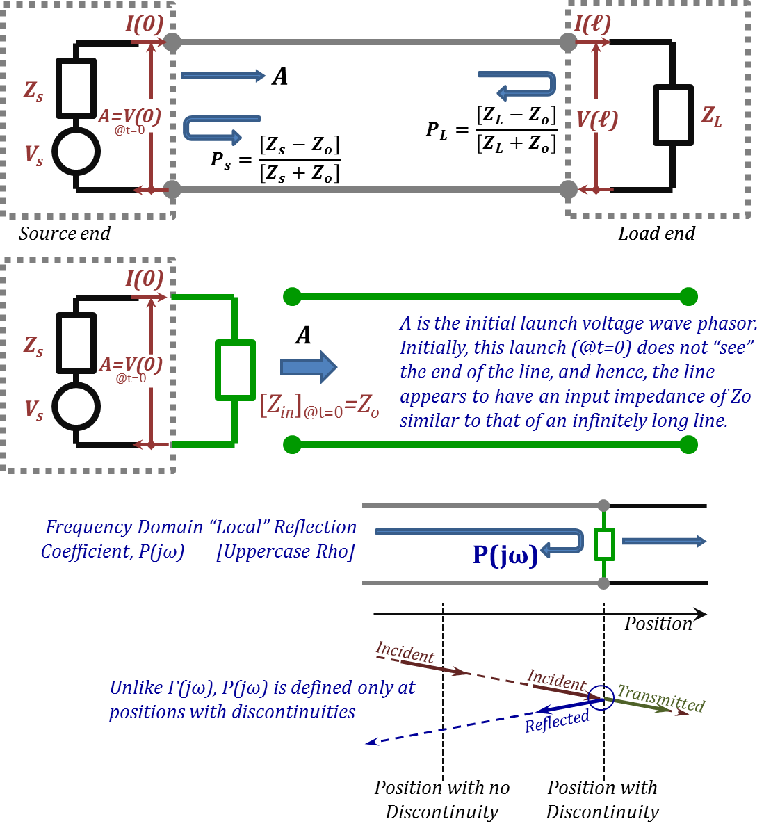
Figure 2.28
Figure 2.28
Referring to Figure 2.28, the "Local" Reflection coefficients $[Ρ(jω) ≡ upper case \text{ }RHO]$ defined at the load and source "discontinuities" are, in general, different from $Γ(jω)$ defined earlier. This local $Ρ(jω)$ is the reflection coefficient at the immediate location of the "discontinuity" assuming no further reflections beyond the current location. Said another way, $Ρ(jω)$ is the "instantaneous" reflection coefficient of the harmonic wave at the time it arrives at a discontinuity not seeing any "future" discontinuities. This is different from $Γ(jω)$ which defines the "steady state" reflection coefficient that accounts for all "past and future" discontinuities. For the example considered in Figures 2.28-2.30, ${{P }_{L}}={{\Gamma }_{L}}\left[ =\mathbf{\Gamma }\left( \ell \right)\text{ }\!\!~\!\text{ }in\text{ }\!~\!\!\text{ }this\text{ }\!\!~\!\text{ }case \right]=\text{ }\!\!~\!\!\text{ }\frac{\left[ {{Z}_{L}}-{{Z}_{o}} \right]}{\left[ {{Z}_{L}}+{{Z}_{o}} \right]}$ since there are no "future" discontinuities beyond the load end of the line.
In the following, we need to refer to both Figures 2.29 and 2.30. The difference between the two figures is that 2.29 shows the multiple reflections at both line ends while 2.30 adds the line signals at an interim location $(z)$. As demonstrated in both figures, the initial launch $(A)$ travels down the TL experiencing modifications in the form of attenuation, ${{e}^{-\alpha z}}$, and phase change, ${{e}^{-j\beta z}}$. So, at location $z$ on the line the modified initial launch will take the form of the phasor $A\cdot {{e}^{-\gamma z}}$ which we will label at $A\!\cdot {{T}_{z}}$, and by the end of the line at $z=\ell $, the phasor will take the form ${{[{{V}^{+}}{{e}^{-\gamma \ell }}]}_{t=\ell /\text{c}}}=A\cdot {{e}^{-\gamma \ell }}=A\cdot T$. This positive traveling wave will bounce off the $Z_{L}$ discontinuity causing a negative $z$-traveling wave at $z=\ell $, viz.,
${{[{{V}^{-}}{{e}^{+\gamma ~\ell }}]}_{t=\ell /c}}={{P }_{L}}\cdot \text{ }\!\!~\!\!\text{ }{{[{{V}^{+}}{{e}^{-\gamma ~\ell }}]}_{t=\ell /c}}={{P }_{L}}\cdot A\cdot T$
The total voltage phasor at that location and at that instant would be
$\text{V}\left( \ell \right)=\text{ }\!\!~\!\!\text{ }{{[{{\text{V}}^{+}}{{\text{e}}^{-\text{ }\gamma\text{ }\ell }}]}_{\text{t}=\ell /\text{c}}}+\text{ }\!\!~\!\!\text{ }{{[{{\text{V}}^{-}}{{\text{e}}^{+\text{ }\gamma\text{ }\ell }}]}_{\text{t}=\ell /\text{c}}}=\text{A}\cdot \text{T}+{{\text{ }\!\!P\!\!\text{ }}_{\text{L}}}\cdot \text{A}\cdot \text{T}=\left[ 1+{{\text{ }\!\!P\!\!\text{ }}_{\text{L}}} \right]\cdot \text{A}\cdot \text{T}$
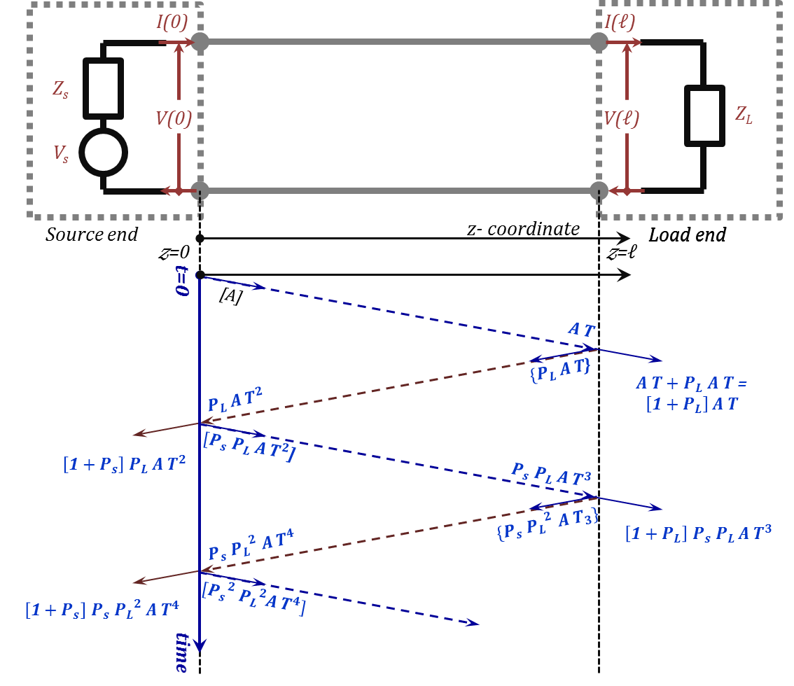
Figure 2.29
Figure 2.29
This is the voltage phasor across the load termination, and hence, we may call it the transmitted voltage phasor (at that location and at that instant). This component will be "absorbed" by the load.
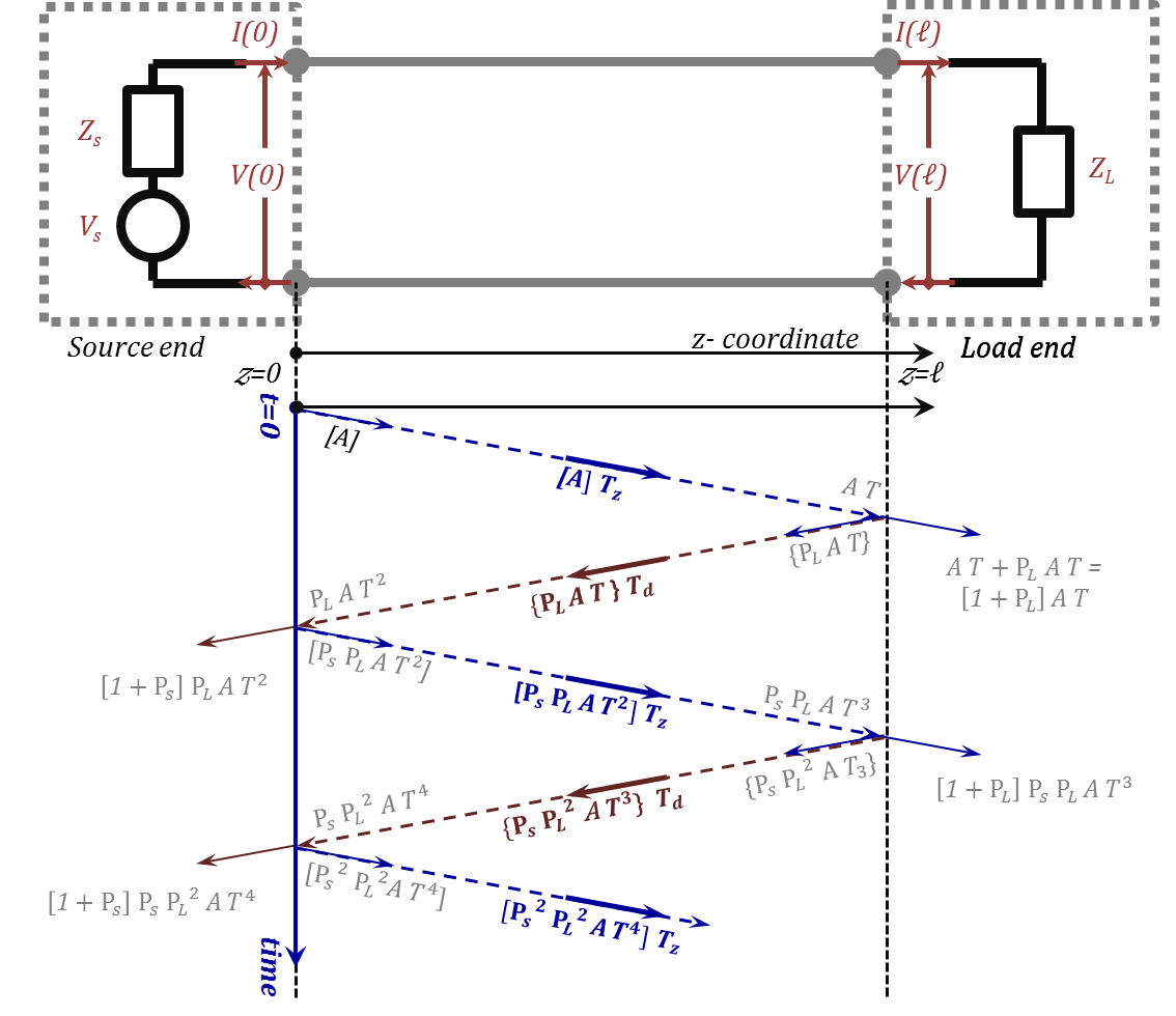
Figure 2.30
$T={{e}^{-~\gamma ~ \ell }}$ $~-~$ ${{T}_{z}}={{e}^{-~\gamma ~ z}}$ $~-~$ ${{T}_{d}}={{e}^{-~\gamma ~ \text{d}}}$ $~-~$ $d=\ell -z$
Figure 2.30
Next, we examine the reflected phasor for the load side. Starting with the ${{[{{V}^{-}}{{e}^{+\gamma ~ \ell }}]}_{t=\ell /\text{c}}}=\{{{P }_{L}}\cdot A\cdot T\}$, this phasor changes through the multiplier ${{e}^{-\gamma ~\cdot ~ distance~traveled}}$, so, at location $z$, the distance traveled would be $d=\ell -z\!\!~\!\!\text{ }$ and at the source end the distance traveled would be $\ell $.
Hence the $–z$ traveling wave will have its phasor expressions as ${{e}^{-\gamma \cdot d}}\cdot \{{{P }_{L}}\cdot A\cdot T\}={{T}_{d}}\cdot \{{{P }_{L}}\cdot A\cdot T\}$ and ${{e}^{-\gamma \cdot \ell }}\cdot \{{{P }_{L}}\cdot A\cdot T\}=T\cdot \{{{P }_{L}}\cdot A\cdot T\}={{P }_{L}}\cdot A\cdot {{T}^{2}}$. This –$z$ wave arrives at the source end at $t=2\ell /\text{c}$. When it does, it will be faced with the discontinuity of the source impedance, causing a reflection and a transmission (similar to what happened at the load end).
The reflection coefficient facing the $–z$ propagation at the source end will be given by $~\!\!\text{ }{{P }_{s}}=\frac{\left[ {{Z}_{s}}-{{Z}_{o}} \right]}{\left[ {{Z}_{s}}+{{Z}_{o}} \right]}$. This makes the reflected and transmitted phasors $[{{P }_{s}}\cdot {{P }_{L}}\cdot A\cdot {{T}^{2}}]\text{ }\!\!~\!\!\text{ }$ and $\left[ \text{1}+{{P }_{s}} \right]\cdot {{P }_{L}}\cdot A\cdot {{T}^{2}}$, respectively. Following the same approach, we can construct the following table, Table 2.3, for the phasor bounce diagram:
$\text{A}={{\text{V}}_{\text{s}}}\cdot \frac{{{\text{Z}}_{\text{o}}}}{\left[ {{\text{Z}}_{\text{s}}}~+~{{\text{Z}}_{\text{o}}} \right]}={{\text{V}}_{\text{s}}}\cdot \frac{\left[ 1-{{\text{ }P\!\!\text{ }}_{\text{s}}} \right]}{2}\tag{2.88}$
Table 2.3
|
@ Source End |
@ location $z$, $\left( \mathbf{d}=\ell -\mathbf{z} \right)$ |
@ Load End |
|||||
|
To $~{ }~{ }{{\mathbf{Z}}_{\mathbf{s}}}$ |
$+z$ Travel |
$+z$ Travel |
$+z$ Travel |
To $~{ }~{ }{{\mathbf{Z}}_{\mathbf{L}}}$ |
|||
|
$-z$ Travel |
$-z$ Travel |
$-z$ Travel |
|||||
|
[$A$] |
${[A]}{{{T}}_{{z}}}$ |
$AT$ |
|||||
|
${{{ }P{ }}_{{L}}}{A}{{{T}}^{2}}$ |
$\{{{{ }P{ }}_{{L}}}{AT}\}{{{T}}_{{d}}}$ |
$\{{{{ }P{ }}_{{L}}}{AT}\}$ |
$\left[ {1}+{{{ }P{ }}_{{L}}} \right]{AT}$ |
||||
|
$\left[ {1}+{{{ }P{ }}_{{s}}} \right]{{{ }P{ }}_{{L}}}{A }~{ }{{{T}}^{2}}$ |
$[{{{ }P{ }}_{{s}}}{{{ }P{ }}_{{L}}}{A }~{ }{{{T}}^{2}}]$ |
$[{{{ }P{ }}_{{s}}}{{{ }P{ }}_{{L}}}{A }~{ }{{{T}}^{2}}]{{{T}}_{{z}}}$ |
${{{ }P{ }}_{{s}}}{ }~{ }{{{ }P{ }}_{{L}}}{A }~{ }{{{T}}^{3}}$ |
||||
|
${{{ }P{ }}_{{s}}}{{{ }P{ }}_{{L}}}^{2}{A }~{ }{{{T}}^{4}}$ |
$\{{{{ }P{ }}_{{s}}}{{{ }P{ }}_{{L}}}^{2}{A }~{ }{{{T}}^{3}}\}{{{T}}_{{d}}}$ |
$\{{{{ }P{ }}_{{s}}}{{{ }P{ }}_{{L}}}^{2}{A }~{ }{{{T}}^{3}}\}$ |
$\left[ {1}+{{{ }P{ }}_{{L}}} \right]{{{ }P{ }}_{{s}}}{{{ }P{ }}_{{L}}}{A }~{ }{{{T}}^{3}}$ |
||||
|
$\left[ {1}+{{{ }P{ }}_{{s}}} \right]{{{ }P{ }}_{{s}}}{ }~{ }{{{ }P{ }}_{{L}}}^{2}{A }~{ }{{{T}}^{4}}$ |
$[{{{ }P{ }}_{{s}}}^{2}{{{ }P{ }}_{{L}}}^{2}{A }~{ }{{{T}}^{4}}]$ |
$[{{{ }P{ }}_{{s}}}^{2}{{{ }P{ }}_{{L}}}^{2}{A }~{ }{{{T}}^{4}}]{{{T}}_{{z}}}$ |
${{{ }P{ }}_{{s}}}^{2}{{{ }P{ }}_{{L}}}^{2}{A }~{ }{{{T}}^{5}}$ |
||||
|
${{{ }P{ }}_{{s}}}^{2}{{{ }P{ }}_{{L}}}^{3}{A }~{ }{{{T}}^{6}}$ |
$\{{{{ }P{ }}_{{s}}}^{2}{{{ }P{ }}_{{L}}}^{3}{A }~{ }{{{T}}^{5}}\}{{{T}}_{{d}}}$ |
$\{{{{ }P{ }}_{{s}}}^{2}{{{ }P{ }}_{{L}}}^{3}{A }~{ }{{{T}}^{5}}\}$ |
$\left[ {1}+{{{ }P{ }}_{{L}}} \right]{{{ }P{ }}_{{s}}}^{2}{{{ }P{ }}_{{L}}}^{2}{A }~{ }{{{T}}^{5}}$ |
||||
|
$\left[ {1}+{{{ }P{ }}_{{s}}} \right]{{{ }P{ }}_{{s}}}^{2}{{{ }P{ }}_{{L}}}^{3}{A }~{ }{{{T}}^{6}}$ |
$[{{{ }P{ }}_{{s}}}^{3}{{{ }P{ }}_{{L}}}^{3}{A }~{ }{{{T}}^{6}}]$ |
$[{{{ }P{ }}_{{s}}}^{3}{{{ }P{ }}_{{L}}}^{3}{A }~{ }{{{T}}^{6}}]{{{T}}_{{z}}}$ |
|||||
|
Phasor Series |
Expression Sum |
||
|
@ Source |
To $~\!\!\text{ }{{\mathbf{Z}}_{\mathbf{s}}}$ |
$\left[ 1+{{\text{ }\!\!P\!\!\text{ }}_{\text{s}}} \right]{{~\text{ }\!\!P\!\!\text{ }}_{\text{L}}}~\text{A}{{\text{T}}^{2}}+\left[ 1+{{\text{ }\!\!P\!\!\text{ }}_{\text{s}}} \right]{{~\text{ }\!\!P\!\!\text{ }}_{\text{s}}}{{~\text{ }\!\!P\!\!\text{ }}_{\text{L}}}^{2}~\text{A}{{\text{T}}^{4}}+\left[ 1+{{\text{ }\!\!P\!\!\text{ }}_{\text{s}}} \right]{{~\text{ }\!\!P\!\!\text{ }}_{\text{s}}}^{2}{{~\text{ }\!\!P\!\!\text{ }}_{\text{L}}}^{3}~\text{A}{{\text{T}}^{6}}+\cdots $ |
$\frac{\left[ 1+{{\text{ }\!P\!\text{ }}_{\text{s}}} \right]{{~\text{ }\!P\!\text{ }}_{\text{L}}}~{{\text{T}}^{~2}}}{\left[ 1-{{\text{ }\!P\!\text{ }}_{\text{s}}}~{{\text{ }\!P\!\text{ }}_{\text{L}}}~{{\text{T}}^{~2}} \right]}\text{A}$ |
|
$-z$ |
${{\text{ }\!\!P\!\!\text{ }}_{\text{L}}}~\text{A}{{\text{T}}^{2}}+{{\text{ }\!\!P\!\!\text{ }}_{~\text{s}}}~{{\text{ }\!\!P\!\!\text{ }}_{\text{L}}}^{2}~\text{A}{{\text{T}}^{4}}+{{\text{ }\!\!P\!\!\text{ }}_{\text{s}}}^{2}{{~\text{ }\!\!P\!\!\text{ }}_{\text{L}}}^{3}~\text{A}{{\text{T}}^{6}}+\cdots $ |
$\frac{{{\text{ }\!P\!\text{ }}_{\text{L}}}~{{\text{T}}^{~2}}}{\left[ 1-{{\text{ }\!P\!\text{ }}_{\text{s}}}~~{{\text{ }\!P\!\text{ }}_{\text{L}}}~{{\text{T}}^{~2}} \right]}\text{A}$ |
|
|
$+z$ |
$\text{A}+{{\text{ }\!\!P\!\!\text{ }}_{\text{s}}}~{{\text{ }\!\!P\!\!\text{ }}_{\text{L}}}~\text{A}{{\text{T}}^{2}}+{{\text{ }\!\!P\!\!\text{ }}_{\text{s}}}^{2}{{~\text{ }\!\!P\!\!\text{ }}_{\text{L}}}^{2}\text{A}{{~\text{T}}^{4}}+[{{\text{ }\!\!P\!\!\text{ }}_{\text{s}}}^{3}~{{\text{ }\!\!P\!\!\text{ }}_{\text{L}}}^{3}~\text{A}{{\text{T}}^{6}}]+\cdots $ |
$\frac{\text{A}}{\left[ 1-{{\text{ }\!\!P\!\text{ }}_{\text{s}}}~{{\text{ }\!P\!\text{ }}_{\text{L}}}{{\text{T}}^{~2}} \right]}$ |
|
|
@ $z$ |
$-z$ |
${{\text{V}}^{-}}\left( z \right)=[{{\text{ }\!\!P\!\!\text{ }}_{\text{L}}}~\text{AT}\left] {{\text{T}}_{\text{d}}}+[{{\text{ }\!\!P\!\!\text{ }}_{\text{s}}}~{{\text{ }\!\!P\!\!\text{ }}_{\text{L}}}^{2}~\text{A}{{\text{T}}^{3}} \right]{{\text{T}}_{\text{d}}}+[{{\text{ }\!\!P\!\!\text{ }}_{\text{s}}}^{2}~{{\text{ }\!\!P\!\!\text{ }}_{\text{L}}}^{3}\text{A}{{\text{T}}^{5}}]{{\text{T}}_{\text{d}}}+\cdots $ |
$\frac{{{\text{ }\!P\!\text{ }}_{\text{L}}}~\text{T }\!~\!\text{ }{{\text{T}}_{\text{d}}}}{\left[ 1-{{\text{ }\!P\!\text{ }}_{\text{s}}}~{{\text{ }\!P\!\text{ }}_{\text{L}}}~{{\text{T}}^{~2}} \right]}\text{A}$ |
|
$+z$ |
${{\text{V}}^{+}}\left( z \right)=\left[ \text{A} \right]{{\text{T}}_{\text{z}}}+\left[ {{\text{ }\!\!P\!\!\text{ }}_{\text{s}}}~{{\text{ }\!\!P\!\!\text{ }}_{\text{L}}}~\text{A}{{\text{T}}^{2}} \right]{{\text{T}}_{\text{z}}}+[{{\text{ }\!\!P\!\!\text{ }}_{\text{s}}}^{2}~{{\text{ }\!\!P\!\!\text{ }}_{\text{L}}}^{2}~\text{A}{{\text{T}}^{4}}]{{\text{T}}_{\text{z}}}+\cdots $ |
$\frac{{{\text{T}}_{\text{z}}}}{\left[ 1-{{\text{ }\!P\!\text{ }}_{\text{s}}}~{{\text{ }\!P\!\text{ }}_{\text{L}}}~{{\text{T}}^{~2}} \right]}\text{A}$ |
|
|
@ Load |
$-z$ |
$[{{\text{ }\!\!P\!\!\text{ }}_{\text{L}}}~\text{AT}\left] +[{{\text{ }\!\!P\!\!\text{ }}_{\text{s}}}~{{\text{ }\!\!P\!\!\text{ }}_{\text{L}}}^{2}~\text{A}{{\text{T}}^{3}} \right]+[{{\text{ }\!\!P\!\!\text{ }}_{\text{s}}}^{2}~{{\text{ }\!\!P\!\!\text{ }}_{\text{L}}}^{3}~\text{A}{{\text{T}}^{5}}]+\cdots $ |
$\frac{{{\text{ }\!P\!\text{ }}_{\text{L}}}~\text{T}}{\left[ 1-{{\text{ }\!P\!\text{ }}_{\text{s}}}~{{\text{ }\!P\!\text{ }}_{\text{L}}}~{{\text{T}}^{~2}} \right]}\text{A}$ |
|
$+z$ |
$\text{AT}+{{\text{ }\!\!P\!\!\text{ }}_{\text{s}}}~{{\text{ }\!\!P\!\!\text{ }}_{\text{L}}}~\text{A}{{\text{T}}^{3}}+{{\text{ }\!\!P\!\!\text{ }}_{\text{s}}}^{2}~{{\text{ }\!\!P\!\!\text{ }}_{\text{L}}}^{2}~\text{A}{{\text{T}}^{5}}+\cdots $ |
$\frac{\text{T}}{\left[ 1-{{\text{ }\!P\!\text{ }}_{\text{s}}}~{{\text{ }\!P\!\text{ }}_{\text{L}}}~{{\text{T}}^{~2}} \right]}\text{A}$ |
|
|
To $~\!\!\text{ }{{\mathbf{Z}}_{\mathbf{L}}}$ |
$\left[ 1+{{\text{ }\!\!P\!\!\text{ }}_{\text{L}}}~ \right]\text{AT}+\left[ 1+{{\text{ }\!\!P\!\!\text{ }}_{\text{L}}}~ \right]{{\text{ }\!\!P\!\!\text{ }}_{\text{s}}}~{{\text{ }\!\!P\!\!\text{ }}_{\text{L}}}~\text{A}{{\text{T}}^{3}}+\left[ 1+{{\text{ }\!\!P\!\!\text{ }}_{\text{L}}}~ \right]\text{ }\!\!P\!\!\text{ }_{\text{s}}^{~~2}~\text{ }\!\!P\!\!\text{ }_{\text{L}}^{~~2}~\text{A}{{\text{T}}^{5}}+\cdots $ |
$\frac{\left[ 1+{{\text{ }\!P\!\text{ }}_{\text{L}}} \right]~\text{T}}{\left[ 1-{{\text{ }\!P\!\text{ }}_{\text{s}}}~{{\text{ }\!P\!\text{ }}_{\text{L}}}~{{\text{T}}^{~2}} \right]}\text{A}$ |
The expressions in the table can be used to construct answers for the voltage phasors as functions of position, i.e.:
At the source end:
${{V}^{+}}=\frac{A}{\left[ 1-{{P }_{s}}~{{P }_{L}}~{{T}^{2}} \right]}=\left\{ {{V}_{s}}\cdot \frac{\left[ 1-{{P }_{s}} \right]}{2}\cdot \frac{1}{\left[ 1-{{P }_{s}}~{{P }_{L}}~{{T}^{2}} \right]} \right\}\tag{2.89}$
${{V}^{-}}=\frac{{{P }_{L}}~\text{ }{{T}^{2}}~A}{\left[ 1~-~{{P }_{s}}~{{P }_{L}}~{{T}^{2}} \right]}=\left\{ {{V}_{s}}\cdot \frac{\left[ 1~-~{{P }_{s}} \right]\text{ }\!\!~\!\!\text{ }}{2}\cdot \frac{1}{\left[ 1~-~{{P }_{s}}~{{P }_{L}}~{{T}^{2}} \right]}\cdot {{P }_{L}}\text{ }\!\!~\!\!\text{ }{{T}^{2}} \right\}={{V}^{+}}\text{ }\!\!~\!\!\text{ }{{P }_{L}}\text{ }\!\!~\!\!\text{ }{{T}^{2}}\tag{2.90}$
$V\left( 0 \right)=\left\{ {{V}^{+}} \right\}+\left\{ {{V}^{-}} \right\}\tag{2.91}$
At location $z$:
${{V}^{+}}\left( z \right)=\frac{{{T}_{z\text{ }}}A}{\left[ 1-{{P }_{s}}~{{P }_{L}}~{{T}^{2}} \right]}=\left\{ {{V}_{s}}\cdot \frac{\left[ 1~-~{{P }_{s}} \right]~\text{ }\!\!~\!\!\text{ }{{T}_{z\text{ }\!\!~\!\!\text{ }}}}{2~\cdot ~\left[ 1~-~{{P }_{s}}~{{P }_{L}}~{{T}^{2}} \right]} \right\}=\left\{ {{V}^{+}} \right\}\cdot {{T}_{z\text{ }\!\!~\!\!\text{ }}}=\left\{ {{V}^{+}} \right\}\cdot {{e}^{-~\gamma ~\cdot~ z}}\tag{2.92}$
${{V}^{-}}\left( z \right)=\frac{{{P }_{L\text{ }~\!\text{ }}}T\text{ }~\!\text{ }{{T}_{d\text{ }~\!\text{ }}}A}{\left[ 1-{{P }_{s}}~{{P }_{L}}~{{T}^{2}} \right]}=\left\{ {{V}_{s}}\cdot \frac{\left[ 1-{{P }_{s}} \right]\text{ }~\!\text{ }{{P }_{L\text{ }~\text{ }}}T\text{ }~\text{ }{{T}_{d\text{ }~\text{ }}}}{2\cdot \left[ 1-{{P }_{s}}~{{P }_{L}}~{{T}^{2}} \right]} \right\}=\left\{ {{V}^{-}} \right\}/{{T}_{z\text{ }~\text{ }}}=\left\{ {{V}^{-}} \right\}\cdot {{e}^{+~\gamma ~\cdot~ z}}\tag{2.93}$
$V\left( z \right)=\left\{ {{V}^{+}} \right\}\cdot {{e}^{-~\gamma ~\cdot~ z}}+\left\{ {{V}^{-}} \right\}\cdot {{e}^{+~\gamma ~\cdot~ z}}\tag{2.94}$
At the load:
$V\left( \ell \right)=\left\{ {{V}^{+}} \right\}\cdot {{e}^{-~\gamma ~\cdot~ \ell }}+\left\{ {{V}^{-}} \right\}\cdot {{e}^{+~\gamma ~\cdot ~\ell }}\tag{2.95}$
It is important to mention that the above obtained expressions for $\left\{ {{\mathbf{V}}^{+}} \right\}\text{ }\!\!~\!\!\text{ and }\!\!~\!\!\text{ }\left\{ {{\mathbf{V}}^{-}} \right\}$ are in agreement with those obtained earlier in Equations (2.41) and (2.42).This can be shown upon the substitution of ${{P }_{s}}=\frac{\left[ {{Z}_{s}}-{{Z}_{o}} \right]}{\left[ {{Z}_{s}}+{{Z}_{o}} \right]}$, ${{P }_{L}}=\frac{\left[ {{Z}_{L}}-{{Z}_{o}} \right]}{\left[ {{Z}_{L}}+{{Z}_{o}} \right]}$, and $\frac{{{\text{V}}_{s}}\text{ }\!~\!\text{ }{{Z}_{o}}}{{{Z}_{s}}+{{Z}_{o}}}={{\text{V}}_{s}}\cdot \frac{\left[ 1-{{P }_{\text{s}}} \right]}{2}$.
- What are the maximum and minimum possible ${SW\!R}$ values on a TL and what is the corresponding magnitude of the reflection coefficient for each?
- For the TL circuit shown in figure 2.17 with parameters: $V_s=10~Volts$, $Z_s=10~Ohm$, $Z_o=50~Ohm$ and $Z_L=25~Ohm$. Using the bounce/multi-reflection analysis, find the magnitude of the first/earliest component travelling in the $+z$ direction.
Return to Lesson
Return to Video
Examples II.4
- For the same circuit as in Exercise 2 above,while replacing the TL with a lossy one having $Z_o=50~Ohm$, $\alpha=0.05 ~dB/wavelength$ and length $2.3$ λ. Using the bounce/multi-reflection analysis, find the magnitude of the first voltage component travelling the $+z$ direction, the first voltage component travelling in the $-z$ direction and the second voltage component travelling in the $+z$ direction at a point $0.5$ λ away from the load. Find the ${SW\!R }$ for each point.
Return to Lesson
Return to Video
Problems II.4
For the same circuit given in Example 1, plot versus distance the magnitude of the first $+z$ component, first $-z$ component and second $+z$ component along the transmission line. Plot the magnitude of the total voltage $(V^+ + V^-)$ along the transmission line.