1. Read the lecture (displayed below) [30-60 minutes]
2. Watch the video  [24:23 minutes]
3. Do the exercises  [~30 minutes]

Total time = [~2:00 hours]

Transmission Line Trace on the Smith Chart:

The Smith chart is a graphical representation that can enable us to monitor the transmission line performance parameters in terms of its $Γ(z)$ and $Z(z)$ at different location of the line. Referring to Figure 2.41, we will demonstrate how the chart can be used to achieve this objective.

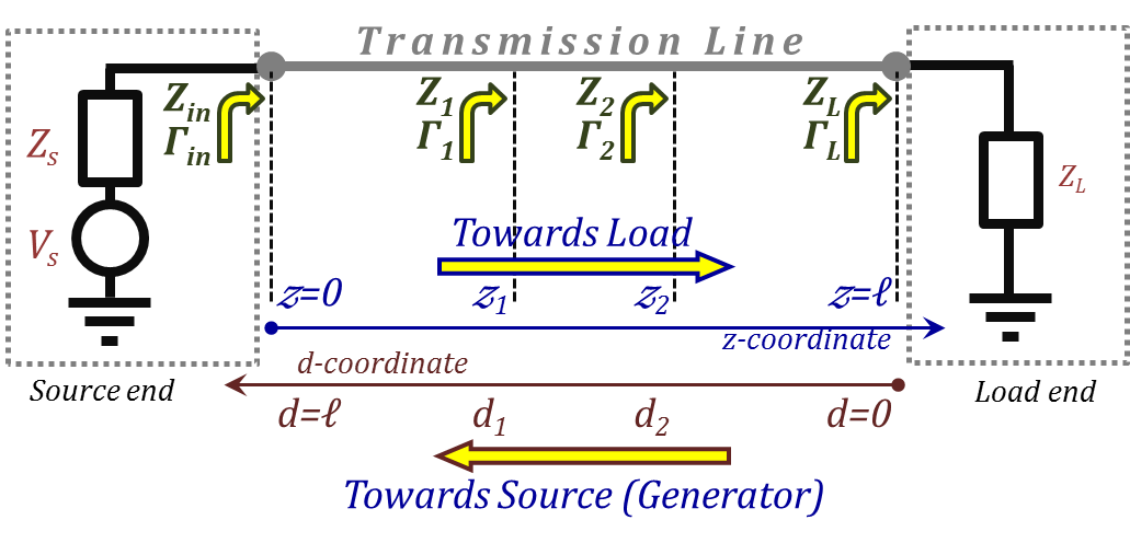
Figure 2.41

Since the chart is a plot of the $Γ$ phasor, then tracking the line trace implies tracing its $Γ(z)$ on the chart. Using Equation (2.105), we can write the expression for the $Γ(z)$ in terms of $Γ(0)$ and $Γ$($\ell $) as:

$\Gamma \left( z \right)=\Gamma \left( 0 \right)\cdot {{e}^{+2~\gamma ~z}}=\Gamma \left( 0 \right)\cdot {{e}^{+2~\alpha ~z}}{{e}^{+2~j~\beta~ z}}=\Gamma \left( 0 \right)\cdot {{e}^{+2~\alpha~ z}}{{e}^{+j~4~\pi~ \left( z/\lambda \right)}}\tag {2.107}$

and,

$\Gamma \left( z \right)={{\Gamma }_{L}}\cdot {{e}^{-2~\gamma~ \left( \ell -z \right)}}={{\Gamma }_{L}}\cdot {{e}^{-2~\alpha~ \left( \ell -z \right)}}~{{e}^{-j~4~\pi~ \cdot~ \left[ \left( \ell -z \right)/\lambda \right]}}$
The latter can be rewritten as a function of d, (the distance from the load end), using $d=ℓ-z$:

$\Gamma \left( d \right)={{\Gamma }_{L}}\cdot {{e}^{-2~\gamma~ d}}={{\Gamma }_{L}}\cdot {{e}^{-2~\alpha ~d}}~{{e}^{-2~j~\beta~ d}}={{\Gamma }_{L}}\cdot {{e}^{-2~\alpha ~d}}~{{e}^{-j~4~\pi~ \cdot~ \left( d/\lambda \right)}}\tag {2.108}$

Equations (2.107) and (2.108) can be rewritten in terms of their magnitude and phase components:

$\left| \Gamma \left( z \right) \right|=\left| \Gamma \left( 0 \right) \right|{{e}^{+2~\alpha~ z}}~~and~\angle \Gamma \left( z \right)=\angle \Gamma \left( 0 \right)+4\pi \cdot \left( z/\lambda \right)\tag {2.109}$

and

$\left| \Gamma \left( d \right) \right|=\left| {{\Gamma }_{L}} \right|{{e}^{-2~\alpha ~d}}~~and~\angle \Gamma \left( d \right)=\angle {{\Gamma }_{L}}-4\pi \cdot \left( d/\lambda \right)\tag {2.110}$

Equations (2.109) and (2.110) are telling us that the magnitude of the $Γ$ phasor changes with position on the line depending on the attenuation coefficient, α. They also show us the continuous (linear) phase change of the phasor.

Case of Lossless TL, $\alpha~=~0$:
In this case, and as can be shown from Equations (2.109) and (2.110), the magnitude of the reflection coefficient is the same (constant) at all line locations:

$\left| \Gamma \left( z \right) \right|=\left| \Gamma \left( 0 \right) \right|=\left| {{\Gamma }_{L}} \right|$

and, hence, the trace of $|Γ(z)|$ is a circle centered at the origin and has a radius of $|Γ(0)|= |Γ_{L}|.$ On the other hand, the phase angle increases as we move towards the load and decreases with motion towards the source. Consequently, the left chart of Figure 2.42 displays the trace of $Γ(z)$ starting at $z=0$, moving towards the load, passing by points $z_{1}$ and $z_{2}$ till the end of the line at $z=ℓ.$ The phase shifts from $z=0$ to $z=z_{1}$, $z=z_{2}$, and finally $z=ℓ$ are represented by angles of counter-clockwise rotations starting at the phase at z=0 in the amounts $4π~(z_{1}/$λ$)$, $4π~(z_{2}/$λ$)$, $4π~(ℓ/$λ$)$, respectively. These rotation angles correspond to rotations of $(z_{1}/$λ$)$, $(z_{2}/$λ$)$, and $(ℓ/$λ$)$, respectively, on the counter-clockwise normalized distance scale labeled "Towards Load".

Likewise, the right chart in Figure 2.42 demonstrates the same line but starting the trace at the load end on the TL. The trace is thus starting at d=0 (z=ℓ), and moves towards the source, passing by points $d_{2}$ $(or~z_{2})$ and $d_{1}$ $(or~z_{1})$ till the source end of the line at $d=ℓ$ $(z=0)$.

The phase shifts from $d=0$ to $d=d_{2}$, $d=d_{1}$, and finally $d=ℓ$ are represented by angles of clockwise rotations in the amounts $4π (d_{2}/$λ$)$, $4π (d_{1}/$λ$)$, $4π (ℓ/$λ$)$, respectively. Again, these rotation angles correspond to rotations of $(d_{2}/$λ$)$, $(d_{1}/$λ$)$, and $(ℓ/$λ$)$, respectively, on the clockwise normalized distance scale labeled "Towards Generator".

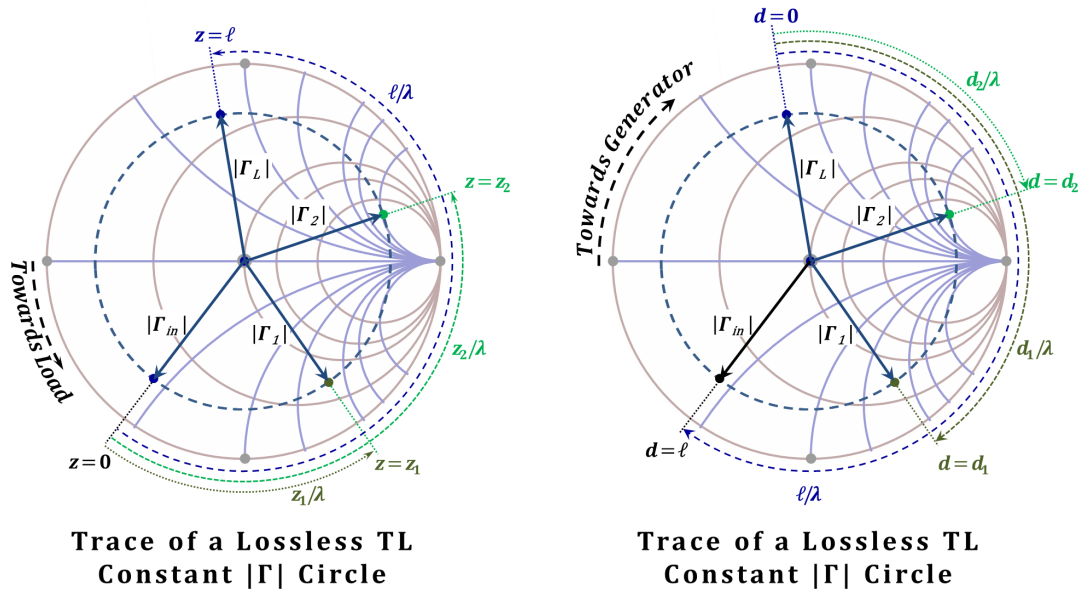
Figure 2.42

Case of Lossy TL, $\alpha~≠~0$:
In this case, and as can be shown from Equations (2.109) and (2.110), the magnitude of the reflection coefficient varies with position, and hence, the $Γ(z)$ is no longer a circle of a constant radius. Varying the magnitude while rotating the phase results in a spiral trace as demonstrated in Figure 2.43. The prescribed spiral pitch depends on the value of the attenuation coefficient. For a low loss line, the pitch is small while it becomes large for larger attenuation coefficients. The spiral trace is inwards as we move towards the source while appearing outwards for motions towards the load.

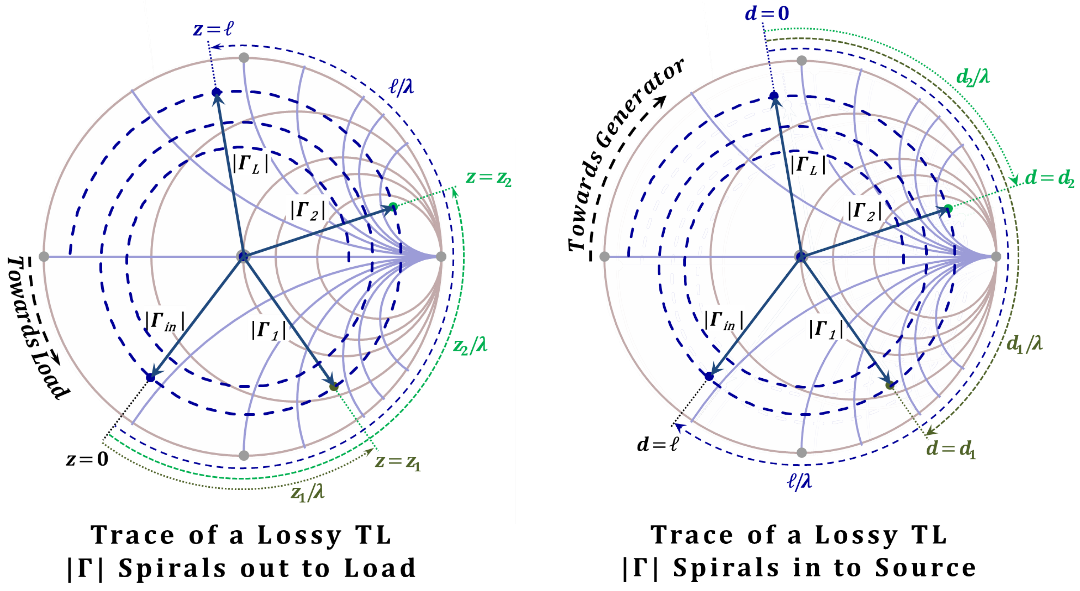
Figure 2.43

Figure 2.43 demonstrates the same TL traces discussed earlier in Figures 2.41 and 2.42 in the presence of line loss, $\alpha~≠~0$.

How Does the Smith Chart Work?

Starting with $Z(z ~or~ d)$:

In this case, we assume that the driving point impedance is known at some point on the line located at a distance $z$ from its source end (distance $d$ from its load end).
The objective is to determine the frequency-domain reflection coefficient at that location. The mathematical expression to be used in this case if we were to do the calculations mathematically is that of Equation (2.46 or 2.101):

$\Gamma \left( z~or~d \right)=\frac{\left[ Z\left( z~or~d \right)-{{Z}_{o}} \right]}{\left[ Z\left( z~or~d \right)+{{Z}_{o}} \right]}$

The Smith chart (graphical) procedure goes as follows, refer to Figure 2.44:

1. Choose a normalization impedance, $Z_{o}$, for the problem at hand. Typically, the characteristic impedance of the "dominant" transmission line of the circuit is a preferred choice.
2. Compute the normalized impedance by dividing $\frac{Z\left( z~or~d \right)}{{{Z}_{o}}}={{Z}_{n}}\left( z~or~d \right)=r+jx$.
3. Locate the "$~r~$" circle for the obtained "$~r~$" value.
4. Locate the "$~x~$" circle for the obtained "$~x~$" value.
5. The intersection of the two circles defines the $\text{ }\!\!\Gamma\!\!\text{ }\left( z~or~d \right)$ point.
6. The line connecting the origin to the $\text{ }\!\!\Gamma\!\!\text{ }\left( z~or~d \right)$ point is the phasor representing$~\text{ }\!\!\Gamma\!\!\text{ }\left( z~or~d \right)$.
7. The length of the $\text{ }\!\!\Gamma\!\!\text{ }\left( z~or~d \right)$ phasor is the magnitude of $\text{ }\!\!\Gamma\!\!\text{ }\left( z~or~d \right)$.
8. Draw a circle centered at the origin passing by the $Γ$ point and project the radius of this circle on the $|Γ|$ scale to read the magnitude of $Γ$.
9. The angle the $\text{ }\!\!\Gamma\!\!\text{ }\left( z~or~d \right)$ phasor makes with the horizontal (real axis) is the angle of the $\text{ }\!\!\Gamma\!\!\text{ }\left( z~or~d \right)$ phasor. Read the phase angle of $Γ$ on the provided angle scale.
10. In rectangular format, the projections of the $\text{ }\!\!\Gamma\!\!\text{ }\left( z~or~d \right)$ phasor on the horizontal and vertical axes are the real and imaginary parts of the $\text{ }\!\!\Gamma\!\!\text{ }\left( z~or~d \right)$ phasor, respectively.

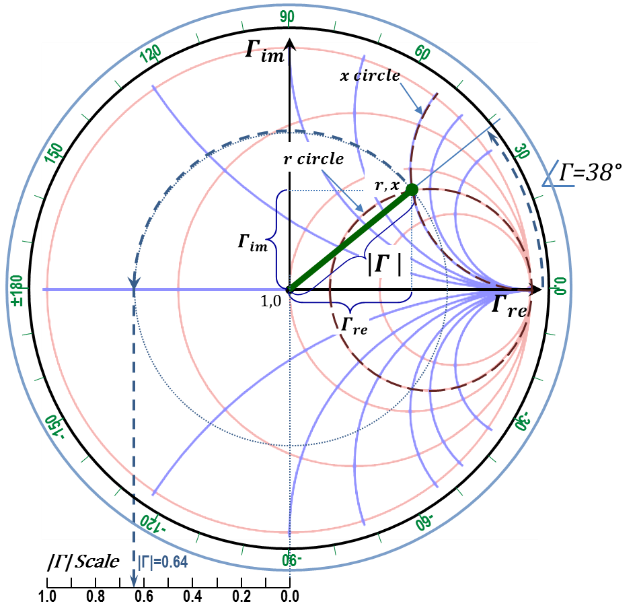
Figure 2.44

Starting with the $\Gamma \left( z~or~d \right)$ phasor:
In this case, we assume that the frequency-domain reflection coefficient is known at some point on the line located at a distance $z$ from its source end (distance $d$ from its load end). The objective is to determine the driving point impedance of the line at that location. The mathematical expression to be used in this case if we were to do the calculations mathematically is that of Equation (2.46 or 101):

$Z\left( z~or~d \right)={{Z}_{o}}\frac{\left[ 1+\Gamma \left( z~or~d \right) \right]}{\left[ 1-\Gamma \left( z~or~d \right) \right]}$

The Smith chart (graphical) procedure goes as follows, again, refer to Figure 2.44:

1. The normalization impedance $Z_{o}$ must be given to us along with the $\text{ }\!\!\Gamma\!\!\text{ }\left( z~or~d \right)$.
2. Locate the $\text{ }\!\!\Gamma\!\!\text{ }\left( z~or~d \right)$ phasor (Magnitude and Phase) or Real and Imaginary.
3. For $|Γ|$, $Γ_{re}$ and $Γ_{im}$ use the $|Γ|$ Scale provided to enter the proper line lengths to be graphed on the chart. For phase, use the phase angle scale to enter the $\angleΓ$.
4. Locate the "$~r~$" circle that passes by the $\text{ }\!\!\Gamma\!\!\text{ }\left( z~or~d \right)$ phasor point – read the value of $r$.
5. Locate the "$~x~$" circle that passes by the $\text{ }\!\!\Gamma\!\!\text{ }\left( z~or~d \right)$ phasor point – read the value of $x$.
6. Compose the obtained $r$ and $x$ values to obtain a numerical value for the complex normalized impedance$~{{Z}_{n}}\left( z~or~d \right)=Z/{{Z}_{o}}=r+jx$.
7. De-normalize ${{Z}_{n}}\left( z~or~d \right)$ to compute the actual driving point impedance of the line $Z\left( z~or~d \right)~$at the position $(z~or~d)$. To de-normalize, you multiply the normalized impedance by the given normalization impedance $Z_{o}$. Thus, $Z\left( z~or~d \right)={{Z}_{n}}\left( z~or~d \right)\cdot {{Z}_{o}}$.

Finding $\Gamma \left( {{z}_{2}}~or~{{d}_{2}} \right)$ (and $Z\left( {{z}_{2}}~or~{{d}_{2}} \right)$) knowing $\Gamma \left( {{z}_{1}}~or~{{d}_{1}} \right)$ or $Z$$\left( {{z}_{1}}~or~{{d}_{1}} \right)$

In this case, we assume that line information (either $Z$ or $Γ$) is known at some point on the line (e.g. $z_{1}$ or $d_{1}$). The objective is to determine the corresponding $Z$ and $Γ$ at another point on the line (e.g. $z_{2}$ or $d_{2}$). The mathematical expressions for this case was given earlier in Equation (2.106), i.e.:

$\left| \Gamma \left( {{z}_{2}} \right) \right|=\left| \Gamma \left( {{z}_{1}} \right) \right|{{e}^{+2~\alpha ~\left( {{z}_{2}}-{{z}_{1}} \right)}}~and~~\angle \Gamma \left( {{z}_{2}} \right)=\angle \Gamma \left( {{z}_{1}} \right)+4\pi \cdot \left[ \left( {{z}_{2}}-{{z}_{1}} \right)/\lambda \right]\tag {2.106}$

Once $Γ(z_{2})$ is determined, we would use Equation (2.46) to get $Z(z_{2})$.

The Smith chart (graphical) procedure is illustrated in Figures 2.45:

1. Locate the line position $z_{1}$ $(or~d_{1}$) on the chart though the $Γ$ Phasor or impedance $Z$ information as demonstrated earlier.

• Moving toward the load, ${{z}_{2}}>{{z}_{1}}$, then according to Equation (2.106), $\left| \text{ }\!\!\Gamma\!\!\text{ }\left( {{z}_{2}} \right) \right|>\left| \text{ }\!\!\Gamma\!\!\text{ }\left( {{z}_{1}} \right) \right|$ and $~\angle \Gamma \left( {{z}_{2}} \right)=\angle \Gamma \left( {{z}_{1}} \right)$
• The corresponding trace for line points on the chart is a counter-clockwise growing spiral. The spiral radius growth is determinedby the exponent$~{{e}^{+2~\alpha ~\left( {{z}_{2}}-{{z}_{1}} \right)}}$. This computation is to be performed manually since the spiral is not part of the chart.
• However, if $~{{z}_{2}}<{{z}_{1}}~\left( or~{{d}_{2}}>{{d}_{1}} \right)$, i.e. we move towards the source (generator), the corresponding motion on the (same) spiral would be in the opposite direction.

2. Compute the normalized distance of rotation $\left[ \left( {{z}_{2}}-{{z}_{1}} \right)/\lambda \right]$ (or $\left[ \left( {{d}_{2}}-{{d}_{1}} \right)/\lambda \right])~$and enter this amount on the chart using the normalized distance scale starting at point "$z_{1}$" to locate point "$z_{2}$".

3. Read $\text{ }\!\!\Gamma\!\!\text{ }\left( {{z}_{2}} \right) (~and~ {{Z}_{n2}}={{r}_{2}}+j{{x}_{2}})$.

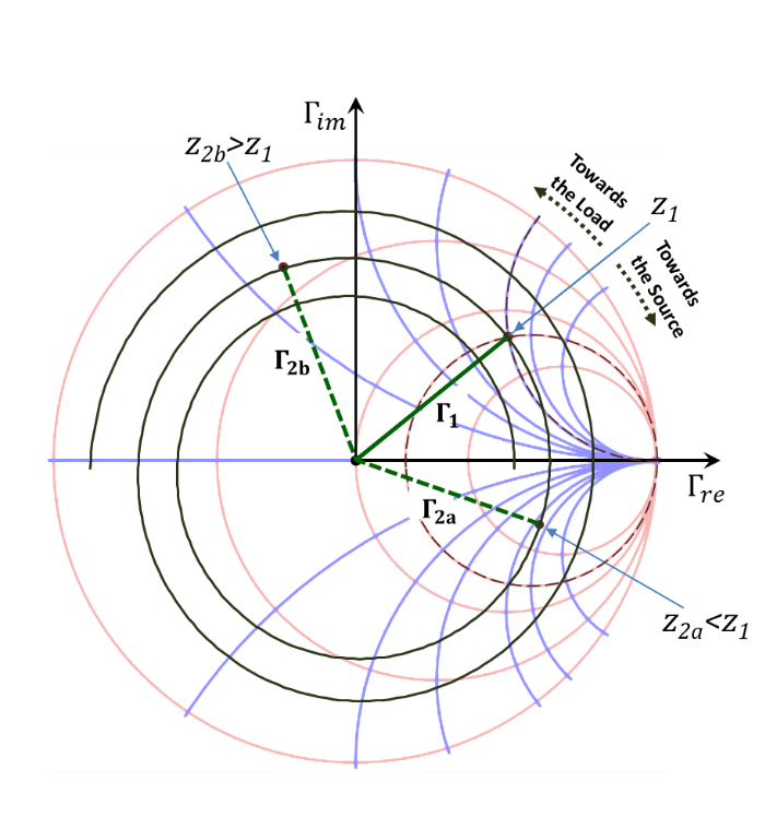
Figure 2.45

Special case (Lossless TL), $\alpha =0:$
This case is similar to the case above except for having a constant radius circle replacing the spiral trace. Figure 2.46 demonstrates the graphical procedure on the chart in a similar manner.

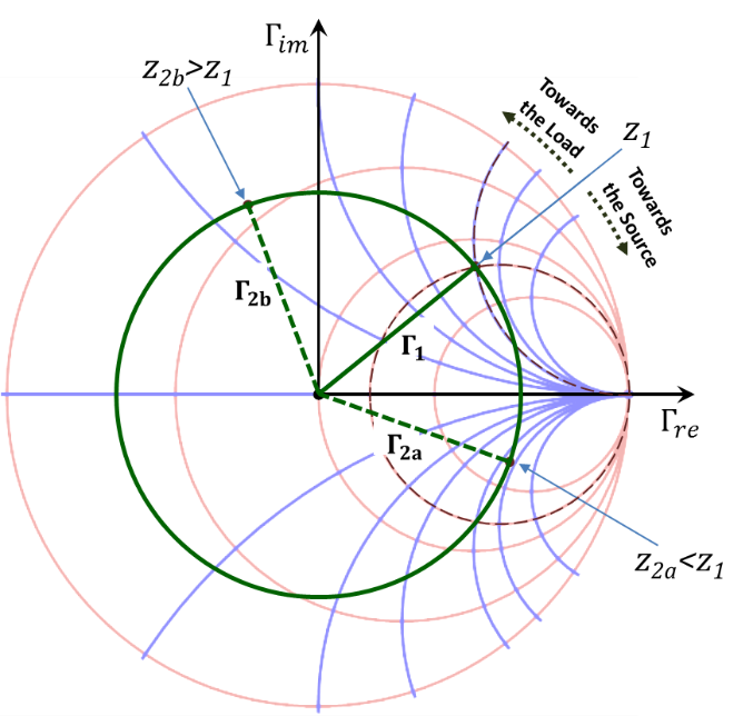
Figure 2.46

Video

1. What is the trace of the reflection coefficient on the Smith chart for a lossless TL of length λ $/~6$ ?
2. What is the trace of the reflection coefficient on the Smith chart for a lossy TL of length λ $/~6$ with an attenuation coefficient of $1\ dB/wave~length$ ?
3. What is the direction of rotation on a Smith chart corresponding to moving along a TL towards the source ?

Return to Lesson

Return to Video

1. For a ${50~Ohm}$ TL of length $0.4$ λ and load ${Z_L=40+j~30~Ohm}$, using the Smith chart find the reflection coefficient at the source.
2. If a load impedance of ${75+j~40~Ohm}$ is connected to a ${50~Ohm}$ TL, find the nearest two locations from the load (in fractions of λ ) to get a purely resistive driving point impedance.
3. For a ${75~Ohm}$ TL terminated with a short circuit, find the locations on the TL where:
1. Driving point impedance is a capacitive reactance of ${j~75~Ohm}$.
2. Driving point impedance is a inductive reactance of ${-j~75~Ohm}$.
3. Magnitude of voltage is maximum.

Return to Lesson

Return to Video

1. A lossless TL is terminated with a ${75~Ohm}$ load. If the ${SWR}$ on the line is ${1.5}$, find the two possible values of the characteristic impedance of the line.
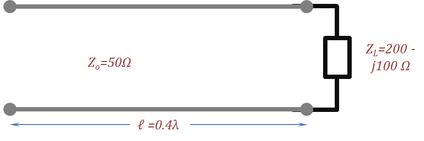
2. For the circuit in the following figure, find the following quantities:
1. ${SWR}$ on the line.
2. Reflection coefficient at the load.
3. Driving point impedance at the input of the line.
4. The nearest voltage minimum to the load.

Return to Lesson

Return to Video

Click here to download the Instructor Guide >>