Chapter II-Lesson 7 of 10 Transmission Lines - Wave Equations
Instructions
- Read the lecture (displayed below) [30-60 minutes]
- Watch the video (21:04 + 2.33 minutes) [30 minutes]
- Do the exercises [~30 minutes]
Total time = [~2:00 hours]
So far, we have been studying the analysis (and design) of transmission line circuits. In the following, we introduce a graphical tool (the Smith Chart) for performing specific analysis and design tasks that is fairly convenient and highly visual. In this regard, it is worth mentioning that even with the advanced computational power that is available to us nowadays, graphical display of the Smith Chart continues to provide a powerful visualization tool that is highly valuable for TL circuit analysis and design.
Addendum E: The Smith Chart:
The Smith Chart:
It was evident from the presentation of the previous sections that the impedance analysis is of prime importance in studying TL performance. However, the corresponding equations looked a bit complicated and are not easy to visualize. TL and RF circuit designers need a tool to enable visual assessment and prediction of problem areas and assessing impedance levels to work on impedance matching problems; such a tool exists and is known as the Smith Chart.
The Smith chart is a graphical tool that maps the impedance values vs. the corresponding reflection coefficient values. Since both are complex numbers, we don't expect a single trace of one vs the other, instead, the Smith chart is composed of multiple traces with parametric variables.
The Smith chart is simply the graph that describes the mathematical relationship between the normalized impedance$~Z\left( z~or~d \right)/{{Z}_{o}}~$ and $~\text{ }\!\Gamma\!\text{ }\left( z~or~d \right)$. Using Equation (2.46), we can write:
${{Z}_{n}}\left( z~or~d \right)=\frac{Z\left( z~or~d \right)}{{{Z}_{o}}}=\frac{\left[ 1~+~\Gamma \text{ }\left( z~or~d \right) \right]}{\left[ 1~-~\Gamma \text{ } \left( z~or~d \right) \right]}$ and $\Gamma \left( z~or~d \right)=\frac{\left[ {{Z}_{n}}\left( z~or~d \right)~-~1 \right]}{\left[ {{Z}_{n}}\left( z~or~d \right)~+~1 \right]} \tag{2.101}$
Spelling out all complex quantities in terms of their real and imaginary components
${{Z}_{n}}\left( z~or~d \right)=\frac{R\left( z~or~d \right)~+~jX\left( z~or~d \right)}{{{Z}_{o}}}=r\left( z~or~d \right)+jx\left( z~or~d \right)$ , and
$\Gamma \left( z~or~d \right)={{\Gamma }_{re}}\left( z~or~d \right)+j~{{\Gamma }_{im}}\left( z~or~d \right)$
By dropping the notation for convenience,
$r+jx=\frac{\left[ 1~+~{{\Gamma }_{re}}~+~j ~{{\Gamma }_{im}} \right]}{\left[ 1~-~{{\Gamma }_{re}}-j ~{{\Gamma }_{im}} \right]}$
Equating both the real and imaginary parts of the above equation yields
$r=\frac{\left[ 1~-~{{\left( {{\Gamma }_{re}} \right)}^{2}}~-~{{\left( {{\Gamma }_{im}} \right)}^{2}} \right]}{\left[ {{\left( 1~-~{{\Gamma }_{re}} \right)}^{2}}~+~{{\left( {{\Gamma }_{im}} \right)}^{2}} \right]}$
$x=\frac{\left[ 2~{{\Gamma }_{im}} \right]}{\left[ {{\left( 1~-~{{\Gamma }_{re}} \right)}^{2}}~+~{{\left( {{\Gamma }_{im}} \right)}^{2}} \right]}$
Manipulation of these two equations yields the following convenient forms:
${{\left[ {{\Gamma }_{re}}-\frac{r}{1+r} \right]}^{2}}+{{\left[ {{\Gamma }_{im}} \right]}^{2}}={{\left[ \frac{1}{1+r} \right]}^{2}}\tag{2.102}$
${{\left[ {{\Gamma }_{re}}-1 \right]}^{2}}+{{\left[ {{\Gamma }_{im}}-\frac{1}{x} \right]}^{2}}={{\left[ \frac{1}{x} \right]}^{2}} \tag{2.103}$
Both equations describe families of circles on a plane formed by ${{\text{ }\!\!\Gamma\!\!\text{ }}_{re}}~$ and $~{{\text{ }\!\!\Gamma\!\!\text{ }}_{im}}$ as its horizontal and vertical axes.
The general circle equation centered at $\left( {{\text{ }\!\!\Gamma\!\!\text{ }}_{re,o}},{{\text{ }\!\!\Gamma\!\!\text{ }}_{im,o}} \right)$ with a radius ${{\text{ }\!\!\Gamma\!\!\text{ }}_{radius}}$ is this plane takes the form:
${{\left[ {{\Gamma }_{re}}-{{\Gamma }_{re,o}} \right]}^{2}}+{{\left[ {{\Gamma }_{im}}-{{\Gamma }_{im,o}} \right]}^{2}}={{\left[ {{\Gamma }_{radius}} \right]}^{2}}$
Hence, for the first Equation (2.102), the "$r$" circles will have their origins located at $\left( \frac{r}{1~+~r},0 \right)$ and the corresponding radius is given by$~\left( \frac{1}{1~+~r} \right)$, while for the "$x$" circles, Equation (2.103), the origins are located at $\left( 1,\frac{1}{x} \right)$ and the corresponding radius is given by $\left( \frac{1}{x} \right)$, see Figure 2.37. In Figure 2.38 shows sets of these circles for various values of $r$ and $x$.
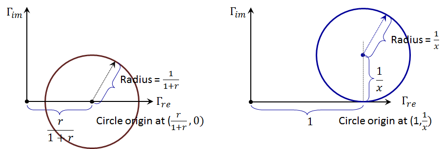
Figure 2.37
Figure 2.37
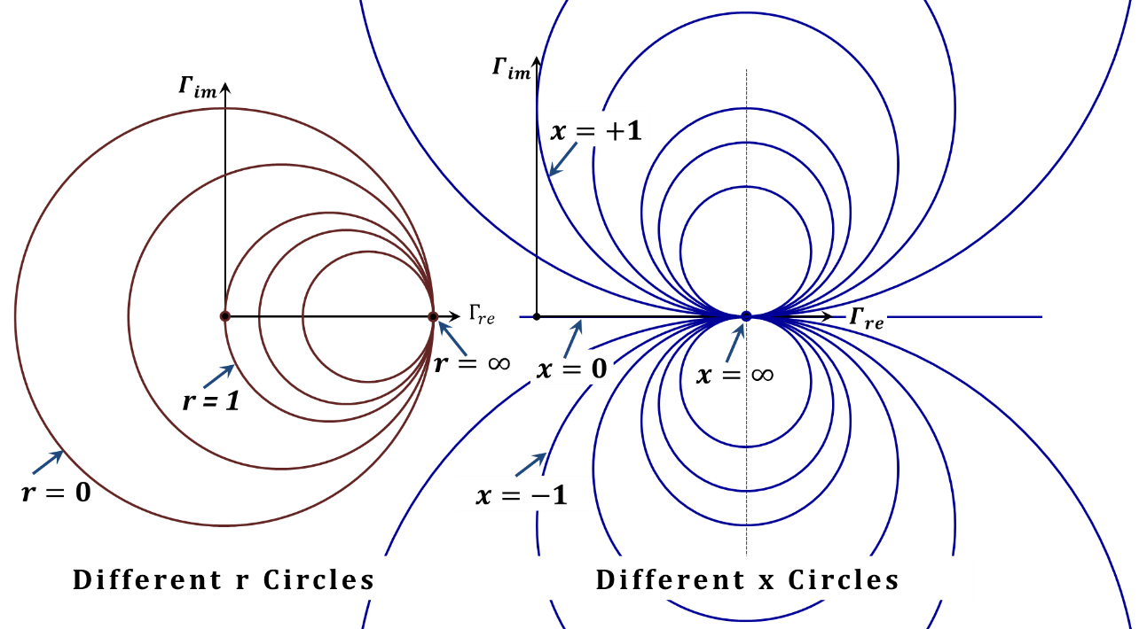
Figure 2.38
Figure 2.38
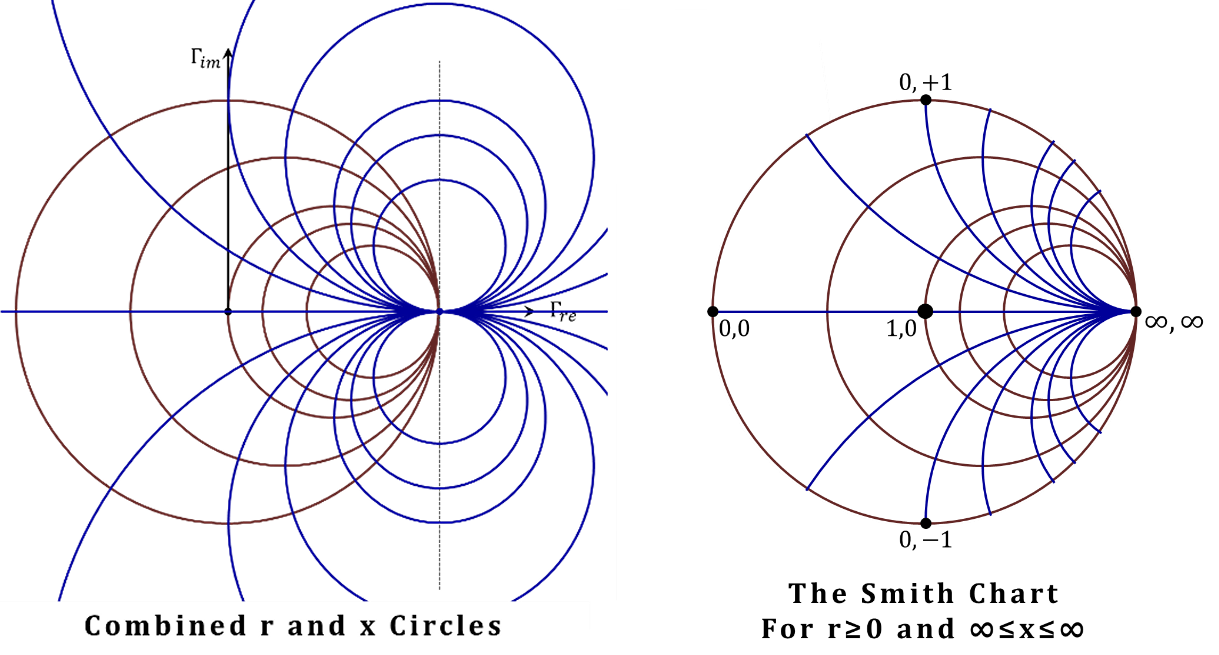
Figure 2.39
Figure 2.39
In the left part of Figure 2.39, both the $r$ and $x$ circles are assembled on the same chart. Finally, the chart on the right is the familiar Smith chart that appears in most prints. In that chart, the parts corresponding to $r<0$ are eliminated.
Scales on the Smith Chart:
There are several scales typically included in a printed Smith chart that can be used to facilitate data entry and extraction. In this section, we will discuss the main scales, which are displayed in Figure 2.40.
- The magnitude of the reflection coefficient ($|Γ|$) scale:
- The phase angle of the reflection coefficient ($\angle \Gamma$) scale:
- Normalized distance moved scale:
The magnitude of $Γ$ is the length of the phasor originating from the origin of the chart and hence is the radius of the circle centered at the origin and passes by the point representing the phasor. The scale for $|Γ|$ is typically positioned on the bottom left of the chart with its zero aligned vertically with the chart origin and has the same "unit length" as that of the "$r=0$" circle. (Note that $r=0$ implies $|Γ|=1$).
To demonstrate the use of this scale, an example of $|Γ|=0.76$ is shown in the figure. From the location of $|Γ|=0.76$ on the scale a vertical line is drawn till it intercepts the horizontal axis of the chart. Next, a circle (centered at the origin) is drawn to pass by the point of interception. Consequently, the radius of this circle is $0.76$, and all points on this circle will have $|Γ|=0.76$.
The phase angle of $Γ$ is the angle the $Γ$ phasor makes with the "horizontal" $Γ_{re}$ axis. The scale for $\angle \Gamma$ is positioned on the outer perimeter of a circle outside the "$r=0$" circle of the chart. The scale is calibrated from $-180°$ to $+180°$ with its zero aligned with the positive side of the horizontal axis of the chart.
To demonstrate the use of this scale, Assume a phase angle of $+72°$ for the $|Γ|=0.76$ example discussed earlier. As shown in the figure, a radial line is placed on the chart for the origin to the $+72°$ mark on the scale. The point of intercept represents the $Γ$ phasor $0.76/+\angle 72°$.
This scale has to do with the relative locations of the $Γ$ phasors corresponding to different locations on the line. Referring to Figure 2.40, $Γ(z_{2})$ and $Γ(z_{1})$ can be related to each other through the use of Equation (2.43):
$\Gamma \left( {{z}_{1}} \right)=\frac{{{V}^{-}}~{{e}^{~+~\gamma {~{z}_~{1}}}}}{{{V}^{+}}~{{e}^{~-~\gamma {~{z}_~{1}}}}}=~\Gamma \left( 0 \right)\cdot {{e}^{~+~2~\gamma {~{z}_~{1}}}} \tag{2.104}$
$\Gamma \left( {{z}_{2}} \right)=\Gamma \left( 0 \right)\cdot {{e}^{~+2~\gamma {~{z}_~{2}}}}=\Gamma \left( {{z}_{1}} \right)\cdot {{e}^{~+~2~\gamma \left( {~{z}_~{2}}-{{z}_{1}} \right)}}\tag {2.105}$
Hence, $\left| \Gamma \left( {{z}_{2}} \right) \right|=\left| \Gamma \left( {{z}_{1}} \right) \right|{{e}^{+2\alpha ~\left( {{z}_{2}}-{{z}_{1}} \right)}}~and~~\angle \Gamma \left( {{z}_{2}} \right)=\angle \Gamma \left( {{z}_{1}} \right)+2\beta \left( {{z}_{2}}-{{z}_{1}} \right)$, or
$\left| \Gamma \left( {{z}_{2}} \right) \right|=\left| \Gamma \left( {{z}_{1}} \right) \right|{{e}^{+2\alpha ~\left( {{z}_{2}}-{{z}_{1}} \right)}}~and~~\angle \Gamma \left( {{z}_{2}} \right)=\angle \Gamma \left( {{z}_{1}} \right)+4\pi \cdot \left[ \frac{\left( {{z}_{2}}-{{z}_{1}} \right)}{\lambda } \right] \tag{2.106}$
Consequently, moving on the line from $z_{1}$ to $z_{2}$ implies a change of the angle of the phasor (rotation) by $4~{ }\pi\text{ }\cdot \left[ \left( {{z}_{2}}-{{z}_{1}} \right)/\text{ }\!\!\lambda\!\!\text{ } \right]$. If $z_{2}>z_{1}$, the change is an increase in the angle and hence a counter-clockwise rotation, and for $z_{2}<z_{1}$, the rotation is clockwise. One can use the phase angle scale to enter these rotations on the chart, however, two normalized distance scales are given to facilitate this process without multiplying the 4π by the $\left[ \left( {{z}_{2}}-{{z}_{1}} \right)/\text{ }\!\!\lambda\!\!\text{ } \right]$. The normalized distance scales provide direct calibration of the $\left[ \left( {{z}_{2}}-{{z}_{1}} \right)/\text{ }\!\!\lambda\!\!\text{ } \right]$ quantity. One of these scales increases counter-clockwise to enable tracking "increasing $z$" locations as we move "towards" the load, while the other scale increases clockwise for tracking "decreasing $z$" locations (increasing $d$) "towards" the source (generator). Both scales are provided along the perimeter of a circle located outside the phase angle scale with the "Towards Generator" scale marked on the outer side of the circle and the "Towards Load" scale marked on the inner side of the circle.
Both scales carry tick marks from $0 ~to~ 0.5$ in a full circle, $360°$. This is because a λ$/2$ distance change correspond to $4\text{ }\pi\text{ }\cdot \left[ \left( {{z}_{2}}-{{z}_{1}} \right)/\text{ }\!\!\lambda\!\!\text{ } \right]=2\text{ }\pi\text{ }\!\!~\!\!\text{ }~~$which is $360°$.
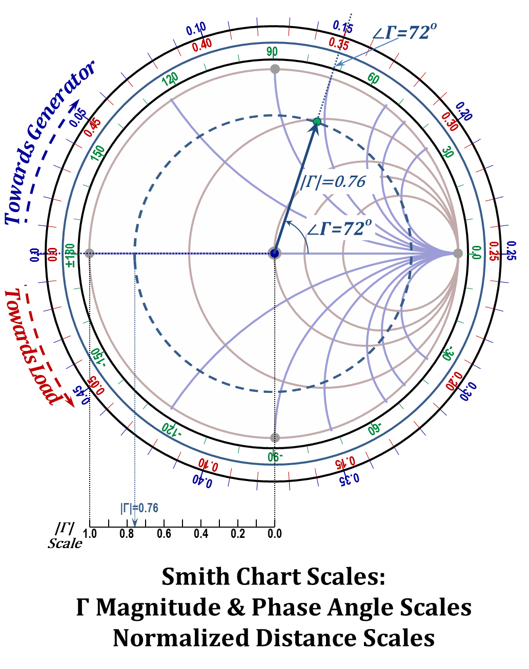
Figure 2.40
Figure 2.40
- What are the two main quantities that are visually related by the Smith chart?
- What does the family of circles radiating in the positive vertical axis direction on the Smith chart represent?
- Explain the lack of circles in the negative horizontal axis direction on the Smith chart?
Return to Lesson
Return to Video
Examples II.7
- Based on the Smith chart, how much TL length is needed so that the reactive part of the translated impedance of any arbitrary load is changed from capacitive to inductive and vice-versa?
- What do the points at coordinates $(1,0)$ and $(-1,0)$ on the Smith chart represent? What is the length of a TL section required to transform one to the other?
Return to Lesson
Return to Video
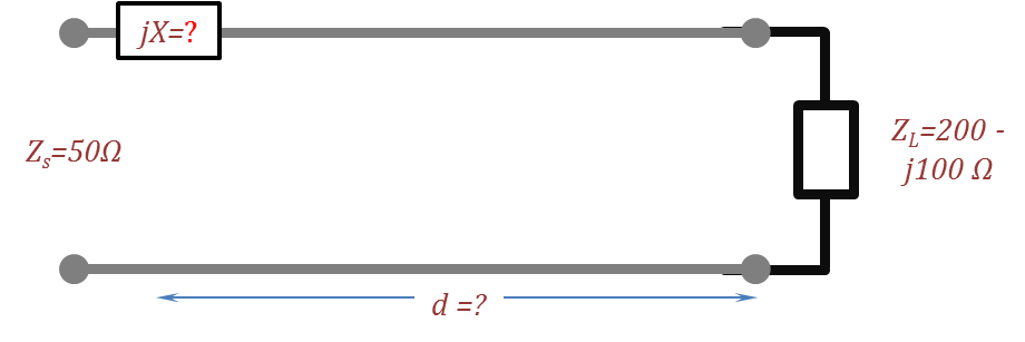
Problems II.7
- For the circuit shown in the following figure, using the Smith chart find the length of the $50~Ohm$ TL section and the series reactance that results in maximum power delivery from a source having internal resistance of $50~Ohm$. Compare your answer to that of Problem II.6.3.