Chapter III-Lesson 1 of 2 Transition to Static Electromagnetics
Instructions
- Read the lecture (displayed below) [30 minutes]
- Watch the video (TBA) [35 minutes]
- Do the exercises [~30 minutes]
Total time = [~1:00 hours]
Introduction
In the previous chapter, we studied the performance of Transmission Lines as circuit elements using an RLCG model. In other words, we used the circuit elements model to study the wave propagation properties of the transmission media. This RLCG model is in fact an approximation and oversimplification of the physical TL configuration. The only way to appreciate this fact is for us to examine how such a model is developed. This will be the topic of the following chapters of this book where we will be studying relevant electromagnetic topics leading to the tools that allow us to determine these "Circuits" model parameters. In the process, we will arrive at more powerful static and dynamic electromagnetic analysis tools. These tools will enable us to study phenomena that are more complex without resorting to the over-simplification of using circuit element modeling.
You see, the issue with the use of approximate models is that you typically cannot predict when the use of these models will fail in yielding reliable results. In the early discussion we had in Chapter I, we showed the need to resort to TL analysis techniques when the size of the components is no longer negligible compared to the wavelength. One can predict as a result that "approximate" circuit model would fail as the frequency goes high. Considering the cases of mm waves and optical waves, it is not practical to represent such cases using Circuits models at all. The only way to deal with these cases is through electromagnetic analysis.
There are other classes of problems that require a decent appreciation of electromagnetic analysis tools. Examples include (but not limited to):
- Antenna analysis and design
- Wireless communication systems and devices
- Semiconductor devices and integrated circuits
- Computer chips (processors, memory, etc.)
- Circuit boards (planar, multilayer, flexible, etc.)
- Cables, connectors, and adaptors
- Discrete components (R, C, L, transformers, etc.)
- Power systems and machines (transformers, motors, generators, etc.)
- Magnetic devices (sensors, relays, actuators, etc.)
- MEMS and MW devices
- RADAR and remote sensing
- Microwave heating and curing
- EMI/EMC analysis
- Nanotechnology
- Photonics
To appreciate the argument we are making here, let us discuss an example of capacitance; one of the fundamental circuit elements that you have learned about before and will be discussed in more detail in later chapters.
A capacitor is simply formed of two conductors isolated from each other by a dielectric (insulator). Physical capacitors that we often see in circuit boards and electrical and electronic devices take many shapes; typical shapes are depicted in Figure 3.1. The figure shows the physical shapes of some "Ceramic Disc" capacitors and next to them is a simplified sketch of their internal physical structure.
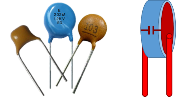
Figure 3.1
Figure 3.1
The typical circuit analysis for such a device is a capacitive circuit element in the nominal capacitance value of the capacitor. Careful analysis shows that such simplified model is not accurate enough for certain applications, especially at high (RF) frequencies. Other "packaging" and "parasitic" elements are present that must be accounted for. Examples are dielectric leakage conductance (G), packaging capacitance ($C_{p}$), lead inductance ($L_{p}$, due to induced magnetic fields), and lead (wire) resistance ($R_{p}$). These are shown in Figure 3.2.
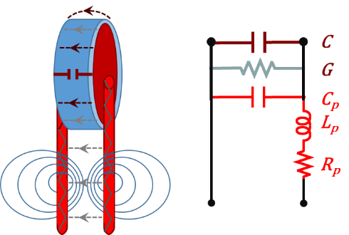
Figure 3.2
Figure 3.2
That being said, to be able to develop the details of such model, we need to understand and relate to the physical phenomenon of resistance, inductance, capacitance, and how the geometrical configuration and material properties among other factors influence their behavior. This is exactly what we are going to "introduce" the learner to in this text book. We use the term "introduce" since the topics involved are far wide and cannot be put all in one book, especially at the introductory level to the subject of EM.
More about the RLCG Parameters
As we recall from past studies of circuit theory, resistance and conductance, are both two sides to the same phenomenon. Both have to do with the ability of the charges to move and the "resistivity" or "conductivity" of the media they move or "flow" in. The conductance is simply the mathematical inverse of the resistance. In this regard, we learned that materials are divided into two main categories: conductors and insulators. A third category was added later in our studies as the "semiconductors" which is by default an insulator that conducts in certain ways under certain conditions. Conductors are those materials that have amble of mobile "free" charges that can move if forced to. The motion of the free charges is known as the electric current. The amount of "impedance" this flow encounters is called the resistance, which depends on the properties of the material and the geometrical configuration and dimensions. The current flow against the resistance causes an electric potential drop and hence power dissipation.
As for the capacitance, it is associated with the presence of an insulating material (dielectric) that isolates two conductor surfaces. The capacitor can be charged (and discharged) by altering the charge amount on the conductor terminals of the capacitor. This, in turn, results in a potential difference across the capacitor terminals which is an indication of energy storage in the capacitor. Energy can be stored (and retrieved) in the capacitor without loss as long as the insulating material is lossless and the two conductors are perfect. An ideal insulating material does not allow direct current flow in a capacitive circuit element. Yet in a dynamic situation, and as a result of charge fluctuations, a dynamic current is modeled in the circuit. We will learn later about this current as the "displacement" current in the dielectric insulator.
The inductance has to do with the magnetic behavior of the media as seen by an electric circuit. Typically, a conductor interaction (linkage) with a medium (magnetic or nonmagnetic) represents an inductance as modeled in the electrical circuit containing that conductor. A time varying current flowing in the inductor results in a potential difference across its terminals while a direct current does not produce any. Both direct and time varying currents result in static and dynamic energy storage in the inductance with no associated dissipation or loss. The inductance value depends on the magnetic (or non-magnetic) properties of the medium, its geometrical configuration and dimensions, as well as the geometrical configuration and dimensions of the conductor (coil) and its shape of interaction (linkage) with the medium.
With all this background information about the Capacitance. Resistance, and Inductance, it is clear that we need to study the electric and magnetic phenomena associated with static and dynamic charges and their interactions with dielectrics, conductors, and magnetic/non-magnetic materials. We will do so in the next few chapters starting with static charges, charges moving with constant velocity generating direct currents, and finally the general case of time varying currents. The first two steps of this study will fall under the "statics" category, while the third one will be under "dynamics".
Before we indulge ourselves in this Static/Dynamic study, we will need to review some mathematical tools that we cannot do without. This review is covered in the Addenda of this chapter, while we start our Statics study in the next chapter, Chapter IV.
Addendum I: Coordinate Systems
Introduction
Coordinate systems are used to define positions/locations in space relative to some arbitrary origin. Three orthonormal coordinates sufficiently define points and locations in three dimensional space. There are three acknowledged coordinate systems in this regard which we will review here in this chapter; they are: the Cartesian, the Cylindrical, and the Spherical coordinate systems.
The Cartesian coordinate system:
The Cartesian coordinate system is the most commonly used as it utilizes three orthonormal constant-direction coordinates. Also, because most of the physical structures are based on rectangular shapes. The convenience of having fixed direction for its three coordinated pays off in many analyses as we will see in our studies in this book and elsewhere.
In Cartesian coordinates, we establish three orthonormal lines/directions/coordinates that stem from an arbitrary origin. Typically, two of these coordinates are laid flat on a horizontal plane; these are typically chosen as the x and y coordinates (see Figure 3.3). A third coordinate is made to emerge orthonormally to the x-y plane and is called the z-coordinate. The positive directions of the three coordinates are chosen to form a right-hand system in the x-y-z-x order (see Figure 3.4). The figure also shows the three unit vectors ${{\vec{a}}_{x}},~{{\vec{a}}_{y}},~and~{{\vec{a}}_{z}}$ for this coordinate system.
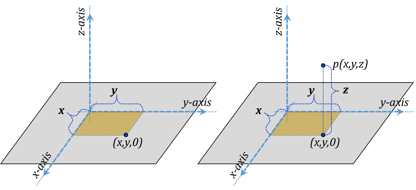
Figure 3.3
Figure 3.3
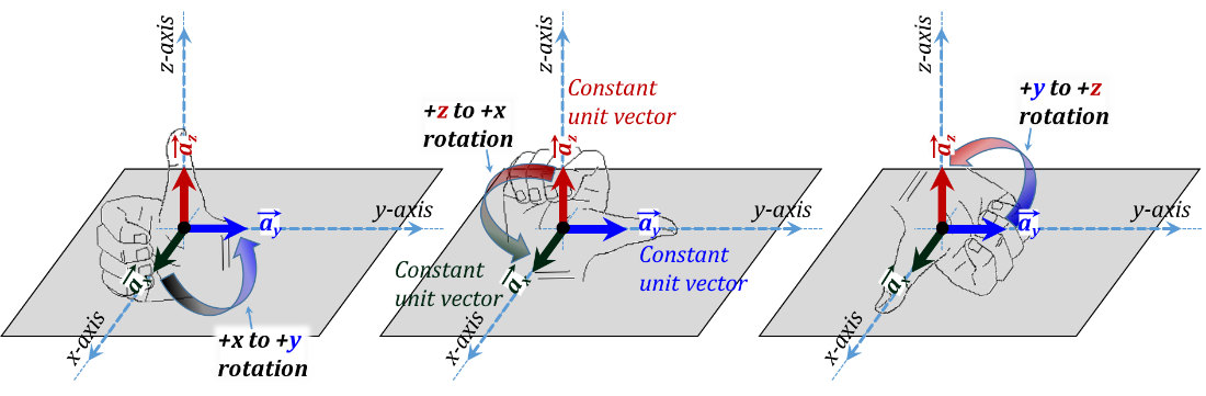
Figure 3.4
Figure 3.4
In the Cartesian coordinate system, a point p is specified by the three coordinates x, y, and z; these are the normal distances between the point p and the y-z plane, z-x plane, and the x-y plane, respectively (Figure 3.5).
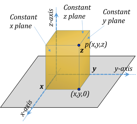
Figure 3.5
Figure 3.5
For integration purposes, incremental elements at p correspond to increasing the coordinate values x, y, and z by Δx, Δy, and Δz, respectively, Figure 3.6. The corresponding volume for the incremental rectangular prism is the product of all three sides Δv = Δx Δy Δz.
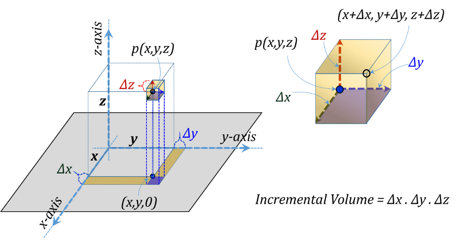
Figure 3.6
Figure 3.6
The vector representation of the three incremental lengths is given in Figure 3.7 while the corresponding three incremental surface area vectors are shown in Figure 3.8. More discussion of vectors will follow in the next Addendum of this chapter.
We need to recognize that the unit vectors ${{\vec{a}}_{x}},~{{\vec{a}}_{y}},~and~{{\vec{a}}_{z}}$ are constant for all points in space for this coordinate system. They are constant in magnitude (which is unity) and constant in directions as well. Length vectors have directions along the lengths themselves, while the direction of an area vector is in the outward normal of the face of that area.
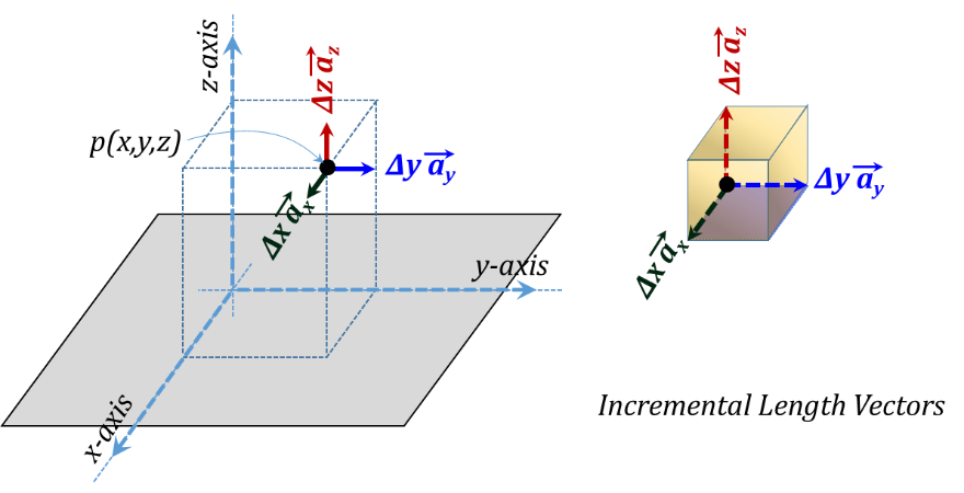
Figure 3.7
Figure 3.7
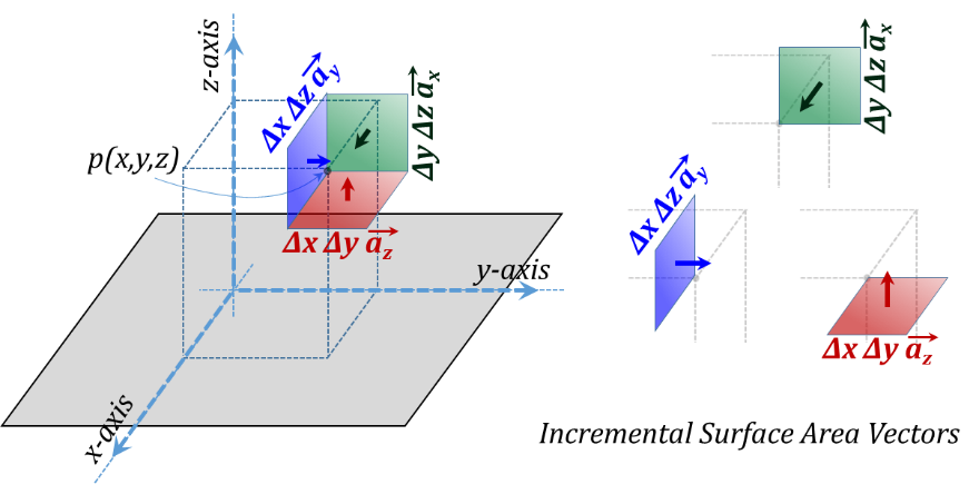
Figure 3.8
Figure 3.8
The Cylindrical coordinate system:
Cylindrical coordinates are useful to express positions and location when a spatial configuration is essentially cylindrical. In this case, Figure 3.9 shows the three orthonormal Cylindrical coordinates ρ, φ, and z as laid over the corresponding Cartesian system chosen with a common z-axis. In this figure, ρ is the radius of a vertical cylinder passing by the position, φ is the angle between the vertical plane containing the z-axis and the position and the z-x plane; finally, z is the height of the position above the x-y plane. The unit vectors along the three coordinates are demonstrated in Figure 3.10. The positive directions of the three coordinates is chosen to form a right-handed system in the ρ-φ-z-ρ order, Figure 3.11.
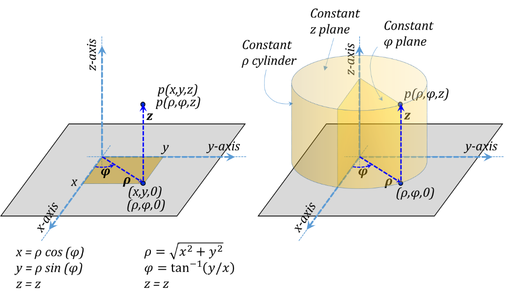
Figure 3.9
Figure 3.9
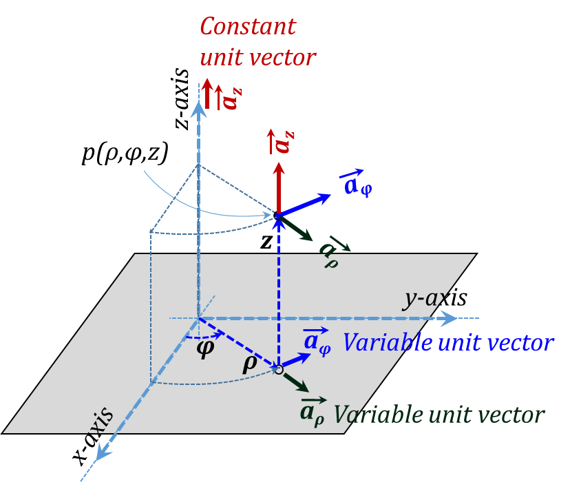
Figure 3.10
Figure 3.10
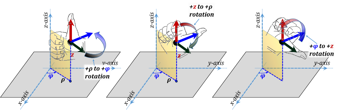
Figure 3.11
Figure 3.11
For integration purposes, incremental elements at p correspond to increasing the coordinate values ρ, φ, and z by Δρ, Δφ, and Δz, respectively, Figure 3.12. The side lengths of the corresponding incremental "rectangular" prism are Δρ, ρΔφ, and Δz, respectively. The corresponding incremental volume is the product of all three sides Δv = Δρ ρΔφ Δz.
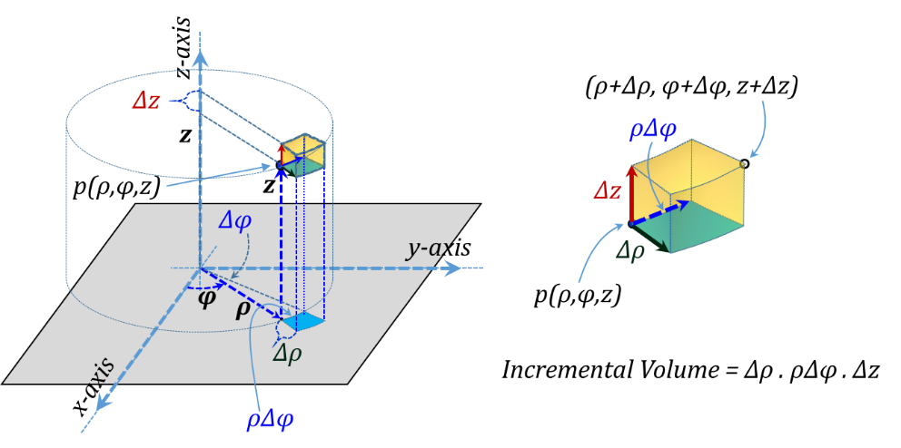
Figure 3.12
Figure 3.12
The vector representation of the three incremental lengths is given in Figure 3.13 while the corresponding three incremental surface area vectors are shown in Figure 3.14. Unlike the case with Cartesian coordinates, the unit vectors ${{\vec{a}}_{\rho }}~and~{{\vec{a}}_{\varphi }}$ are variable vectors as they both vary in direction as we move around in space. However, the unit vector ${{\vec{a}}_{z}}$ is the same as that of Cartesian coordinates and hence is a constant vector for all points in space.
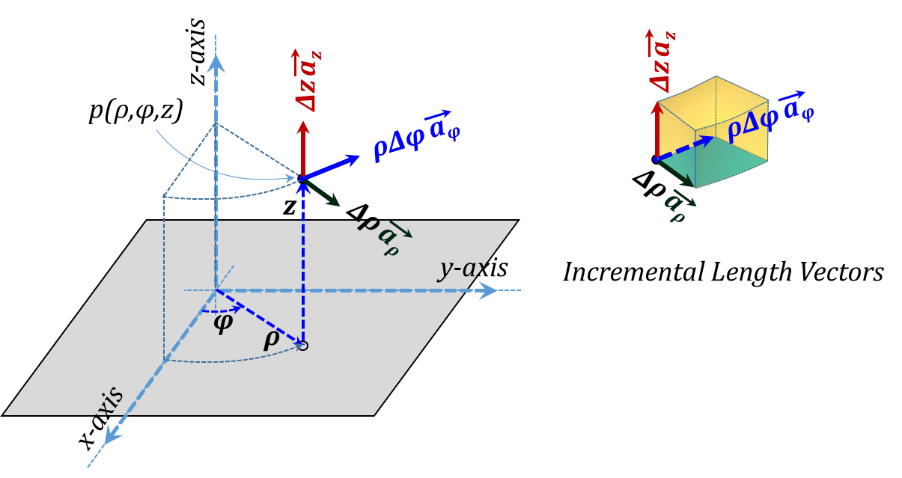
Figure 3.13
Figure 3.13
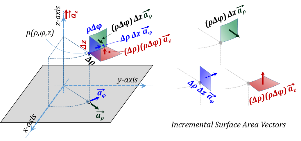
Figure 3.14
Figure 3.14
The Spherical coordinate system:
Spherical coordinates are typically used in cases where a spatial configuration is essentially spherical. The three orthonormal Spherical coordinates are r, θ, and φ, see Figure 3.15. This figure shows all three coordinate systems simultaneously in order to demonstrate their relationship to each other.
As shown in the figure, r is the radius of a sphere passing by the position p while being concentric with the origin. The angle θ is the second coordinate parameter and is the angle between the radial line connecting the position to the origin and the z-axis. The angle θ can also be defined as the angle of the cone whose head is the origin, coaxial with the z-axis and passing by the position p. Finally, the angle φ is the same as defined for Cylindrical coordinates, i.e., the angle between the vertical plane containing the z-axis and the position p and the z-x plane.
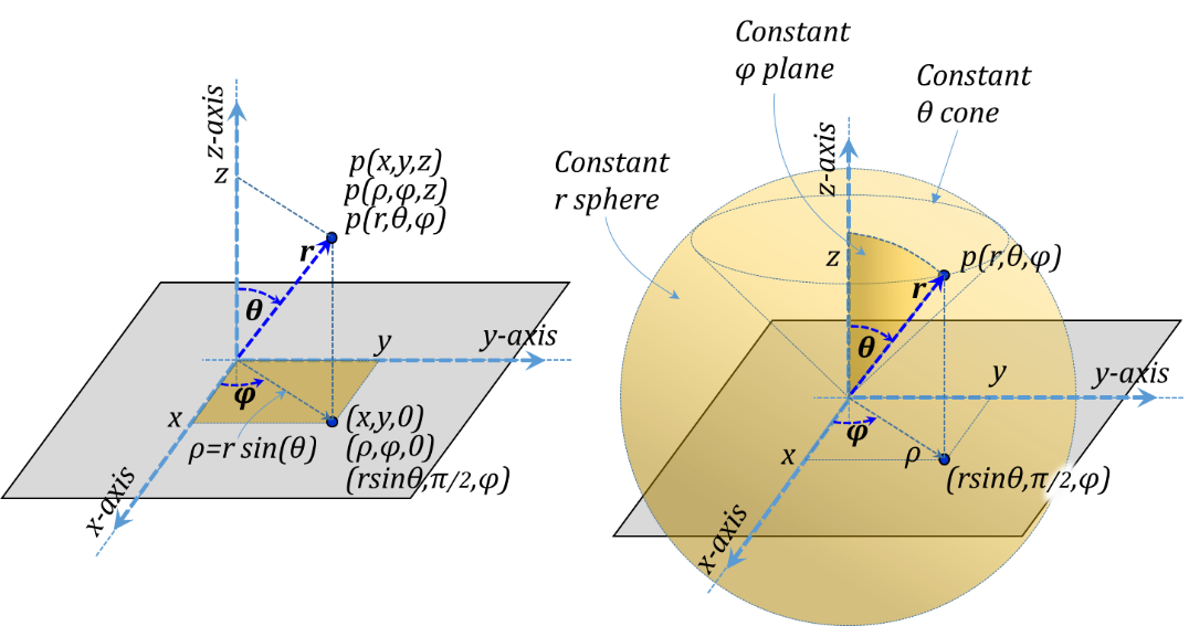
Figure 3.15
Figure 3.15
In Figure 3.16, we demonstrate the three orthonormal unit vectors$~{{\vec{a}}_{r}}~,~{{\vec{a}}_{\theta }},~and~{{\vec{a}}_{\varphi }}$. Again, the positive directions of the three coordinates is chosen to form a right-handed system in the r-θ-φ-r order, Figure 3.17.
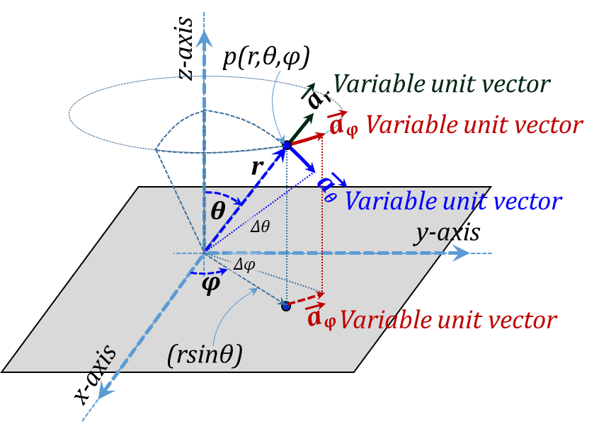
Figure 3.16
Figure 3.16
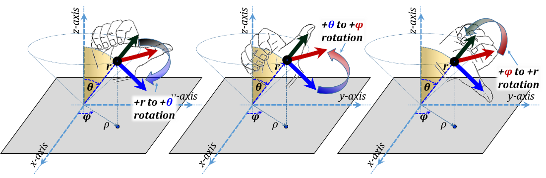
Figure 3.17
Figure 3.17
For integration purposes, incremental elements at p correspond to increasing the coordinate values r, θ, and φ by Δr, Δθ, and Δφ, respectively, Figure 3.18. The side lengths of the corresponding incremental "rectangular" prism are Δr, rΔθ, and rsin(θ)Δφ, respectively. The corresponding incremental volume is the product of all three sides Δv = Δr rΔθ rsin(θ)Δφ.
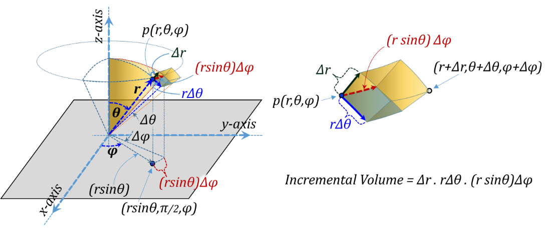
Figure 3.18
Figure 3.18
The vector representation of the three incremental lengths is given in Figure 3.19 while the corresponding three incremental surface area vectors are shown in Figure 3.20. Needless to say, all three unit vectors ${{\vec{a}}_{r}},{{\vec{a}}_{\theta }},~and~{{\vec{a}}_{\varphi }}$ are variable vectors as they all vary in direction as we move around in space.
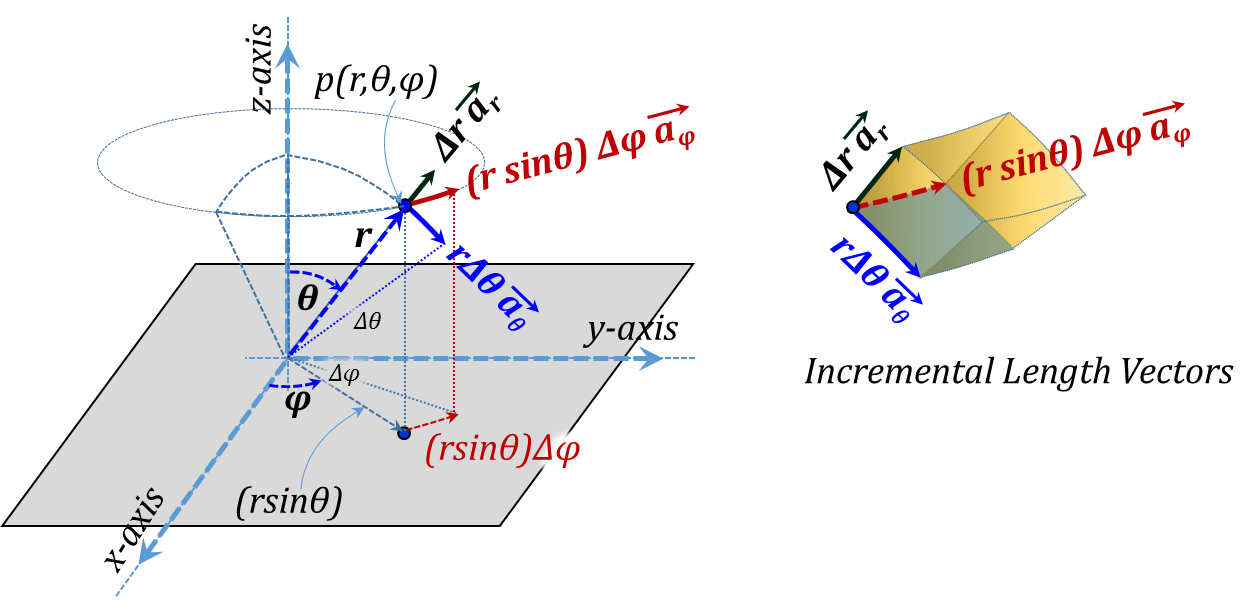
Figure 3.19
Figure 3.19
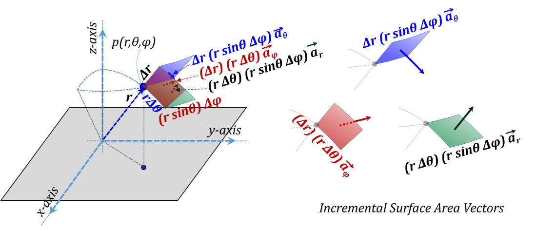
Figure 3.20
Figure 3.20
Relationships between Coordinate Systems:
Frequently, in the course of analytical procedures, we would be faced with the need to convert from one coordinate system to another. Typically, the conversion would be needed between Cylindrical and Cartesian and between Spherical and Cartesian. In some cases this is needed for convenience in carrying out a "difficult" integration or to identify with a specific coordinate-related phenomenon. However, in many cases it is done to avoid dealing with variable unit vectors. Converting to Cartesian coordinates replaces the variable unit vectors with constant ones that facilitates integration procedures involving vectors.
Examining Figures 3.9 and 3.10 for Cylindrical coordinates and 3.14 and 3.15 for Spherical coordinates, we can write down the relationships for the coordinate parameters and the corresponding unit vectors as laid down in the tables below.
Table 3.1 - Coordinate Relations
Table 3.2 - Unit vectors Relations
|
Cylindrical – Cartesian |
Spherical – Cartesian |
Cylindrical - Spherical |
|
$\overrightarrow{{{a}_{\rho }}}=\cos \varphi ~\overrightarrow{{{a}_{x}}}+\sin \varphi ~\overrightarrow{{{a}_{y}}}$ $\overrightarrow{{{{a}}_{{ }\varphi{ }}}}=-\sin { }\varphi{ }~{ }\overrightarrow{{{{a}}_{{x}}}}+\cos { }\varphi{ }~{ }\overrightarrow{{{{a}}_{{y}}}}$ $\overrightarrow{{{{a}}_{{z}}}}=\overrightarrow{{{{a}}_{{z}}}}$ |
$\overrightarrow{{{{a}}_{{r}}}}=\sin { }\theta{ }\cos { }\varphi{ }~{ }\overrightarrow{{{{a}}_{{x}}}}+\sin { }\theta{ }\sin { }\varphi{ }~{ }\overrightarrow{{{{a}}_{{y}}}}+\cos { }\theta{ }\overrightarrow{{{{a}}_{{z}}}}$ $\overrightarrow{{{{a}}_{{ }\theta{ }}}}=\cos { }\theta{ }\cos { }\varphi{ }~{ }\overrightarrow{{{{a}}_{{x}}}}+\cos { }\theta{ }\sin { }\varphi{ }~{ }\overrightarrow{{{{a}}_{{y}}}}-\sin { }\theta{ }\overrightarrow{{{{a}}_{{z}}}}$ $\overrightarrow{{{{a}}_{{ }\varphi{ }}}}=-\sin { }\varphi{ }~{ }\overrightarrow{{{{a}}_{{x}}}}+\cos { }\varphi{ }~{ }\overrightarrow{{{{a}}_{{y}}}}$ |
${{{\vec{a}}}_{{r}}}={{{\vec{a}}}_{{ }\rho{ }}}\sin { }\theta{ }+{{{\vec{a}}}_{{z}}}\cos { }\theta{ }$ ${{{\vec{a}}}_{{ }\theta{ }}}={{{\vec{a}}}_{{ }\rho{ }}}\cos { }\theta{ }-{{{\vec{a}}}_{{z}}}\sin { }\theta{ }$ $\overrightarrow{{{{a}}_{{ }\varphi{ }}}}=\overrightarrow{{{{a}}_{{ }\varphi{ }}}}$ |
|
$\overrightarrow{{{{a}}_{{x}}}}=\cos { }\varphi{ }~{ }\overrightarrow{{{{a}}_{{ }\rho{ }}}}-\sin { }\varphi{ }~{ }\overrightarrow{{{{a}}_{{ }\varphi{ }}}}$ $\overrightarrow{{{{a}}_{{y}}}}=\sin { }\varphi{ }~{ }\overrightarrow{{{{a}}_{{ }\rho{ }}}}+\cos { }\varphi{ }~{ }\overrightarrow{{{{a}}_{{ }\varphi{ }}}}$ $\overrightarrow{{{{a}}_{{z}}}}=\overrightarrow{{{{a}}_{{z}}}}$ |
$\overrightarrow{{{{a}}_{{x}}}}=\sin { }\theta{ }\cos { }\varphi{ }~{ }\overrightarrow{{{{a}}_{{r}}}}+\cos { }\theta{ }\cos { }\varphi{ }~{ }\overrightarrow{{{{a}}_{{ }\theta{ }}}}-\sin { }\varphi{ }\overrightarrow{{{{a}}_{{ }\varphi{ }}}}$ $\overrightarrow{{{{a}}_{{y}}}}=\sin { }\theta{ }\sin { }\varphi{ }~{ }\overrightarrow{{{{a}}_{{r}}}}+\cos { }\theta{ }\sin { }\varphi{ }~{ }\overrightarrow{{{{a}}_{{ }\theta{ }}}}+\cos { }\varphi{ }\overrightarrow{{{{a}}_{{ }\varphi{ }}}}$ $\overrightarrow{{{{a}}_{{z}}}}=\cos { }\theta{ }\overrightarrow{{{{a}}_{{r}}}}-\sin { }\theta{ }\overrightarrow{{{{a}}_{{ }\theta{ }}}}$ |
${{{\vec{a}}}_{{ }\rho{ }}}={{{\vec{a}}}_{{r}}}\sin { }\theta{ }+{{{\vec{a}}}_{{ }\theta{ }}}\cos { }\theta{ }$ ${{{\vec{a}}}_{{z}}}={{{\vec{a}}}_{{r}}}\cos { }\theta{ }-{{{\vec{a}}}_{{ }\theta{ }}}\sin { }\theta{ }$ $\overrightarrow{{{{a}}_{{ }\varphi{ }}}}=\overrightarrow{{{{a}}_{{ }\varphi{ }}}}$ |
Vector Expressions:
Also, for a vector ${\vec{F}}$ expressed in Cartesian, Cylindrical and Spherical coordinates as:
$\vec{F}={{F}_{x}}~{{\vec{a}}_{x}}+{{F}_{y}}~{{\vec{a}}_{y}}+{{F}_{z}}~{{\vec{a}}_{z}},$
${\vec{F}}={{{F}}_{{ }\rho{ }~{ }}}{{{\vec{a}}}_{{ }\rho{ }}}+{{{F}}_{{ }\varphi{ }}}{ }~{ }{{{\vec{a}}}_{{ }\varphi{ }}}+{{{F}}_{{z}}}{ }~{ }{{{\vec{a}}}_{{z}}},$
${\vec{F}}={{{F}}_{{r }~{ }}}{{{\vec{a}}}_{{r}}}+{{{F}}_{{ }\theta{ }~{ }}}{{{\vec{a}}}_{{ }\theta{ }}}+{{{F}}_{{ }\varphi{ }}}{ }~{ }{{{\vec{a}}}_{{ }\varphi{ }}}$
Table 3.3 – Vector Expression Relations
|
Cylindrical to Cartesian |
Spherical to Cartesian |
|
${{{F}}_{{ }\rho{ }}}={{{F}}_{{x}}}\cos { }\varphi{ }+{{{F}}_{{y}}}\sin { }\varphi{ }$ ${{{F}}_{{ }\varphi{ }}}=-{{{F}}_{{x}}}\sin { }\varphi{ }+{{{F}}_{{y}}}\cos { }\varphi{ }$ ${{{F}}_{{z}}}={{{F}}_{{z}}}$ |
${{{F}}_{{r}}}={{{F}}_{{x}}}{ }~{ sin }\theta{ }~{ cos }\varphi{ }+{{{F}}_{{y}}}{ }~{ sin }\theta{ }~{ sin }\varphi{ }+{{{F}}_{{z}}}{ }~{ cos }\theta{ }$ ${{{F}}_{\vartheta }}={{{F}}_{{x}}}{ }~{ cos }\theta{ }~{ cos }\varphi{ }+{{{F}}_{{y}}}{ }~{ cos }\theta{ }~{ sin }\varphi{ }-{{{F}}_{{z}}}{ }~{ sin }\theta{ }$ ${{{F}}_{{ }\varphi{ }}}=-{{{F}}_{{x}}}{ }~{ sin }\varphi{ }+{{{F}}_{{y}}}{ }~{ cos }\varphi{ }$ |
|
${{{F}}_{{x}}}={{{F}}_{{ }\rho{ }}}{ }~{ cos }\varphi{ }-{{{F}}_{{ }\varphi{ }}}\sin { }\varphi{ }$ ${{{F}}_{{y}}}=-{{{F}}_{{ }\rho{ }}}{ }~{ sin }\varphi{ }+{{{F}}_{{ }\varphi{ }}}\cos { }\varphi{ }$ ${{{F}}_{{z}}}={{{F}}_{{z}}}$ |
${{{F}}_{{x}}}={{{F}}_{{r}}}{ }~{ sin }\theta{ }~{ cos }\varphi{ }+{{{F}}_{{ }\theta{ }}}{ }~{ cos }\theta{ }~{ cos }\varphi{ }-{{{F}}_{{ }\varphi{ }}}{ }~{ sin }\varphi{ }$ ${{{F}}_{{y}}}={{{F}}_{{r}}}{ }~{ sin }\theta{ }~{ sin }\varphi{ }+{{{F}}_{{ }\theta{ }}}{ }~{ cos }\theta{ }~{ sin }\varphi{ }+{{{F}}_{{ }\varphi{ }}}{ }~{ cos }\varphi{ }$ ${{{F}}_{{z}}}={{{F}}_{{r}}}{ }~{ cos }\theta{ }-{{{F}}_{{ }\theta{ }}}{ }~{ sin }\theta{ }$ |
- Mention some engineering areas that rely on EM analysis tools?
- Draw the complete circuit model of a practical capacitor?
- Which fundamental physical phenomenon corresponds to a capacitor circuit component? Which fundamental physical phenomenon corresponds to an inductor circuit component?
Return to Lesson
Return to Video
Examples III.1
- Convert the vector $10\,{{\vec{a}}_{x}}+4\,{{\vec{a}}_{y}}-3\,{{\vec{a}}_{z}}$ to both cylindrical and spherical coordinates?
- Convert the vector $(2,1,2)$ given in cylindrical coordinates to rectangular coordinates at the two point locations $(1,-1,0)$ and $(1,1,0)$.
- Convert the vector $(2,3,2)$ given in spherical coordinates to rectangular coordinates at the two point locations $(1,-1,0)$ and $(1,1,0)$.
Return to Lesson
Return to Video
Problems III.1
- A field is given as $\vec{G}=[25/({{x}^{2}}+{{y}^{2}})][x\,{{\vec{a}}_{x}}+y\,{{\vec{a}}_{y}}]$. Find the unit vector in the direction of ${\vec{G}}$ at a point $(3,4,-2)$.
- Find the volume of the portion of the cylinderical shell which falls in the region $x>0$, $y>0$, $3<\rho <4$ and $|z|<1$.
- Find the volume of the portion of a ball (solid sphere) or radius ${5~m}$ that falls in the region $x>0$, $y>0$, $\left| z \right|<3$.