Chapter II-Lesson 10 of 10 Transmission Lines - Wave Equations
Instructions
- Read the lecture (displayed below) [30-60 minutes]
- Watch the video [10:05 minutes]
- Do the exercises [~30 minutes]
Total time = [~1:45 hours]
In this lecture, we will learn about how to use the Smith Chart to design a single stub (tuner) matching.
In Lecture II.6, we learned about stub matching. Figure 2.25 demonstrates the configuration for stub matching using a short circuited stub in two possible arrangements connected to the main line both in series and in parallel. Two other arrangements using open circuited stubs instead are possible as well. Hence, we can say that there are four options in the stub matching design problem.
In fact, there are more options that we have not mentioned in this design problem:
1.The stub reactance/susceptance whether inductive or capacitive adds other degrees of freedom (options) in the design process. This doubles the above mentioned four possibilities yielding eight possible design solutions.
2. Another obvious option is the choice of line to be used as a stub. Ideally, this should be a lossless line, and typically assumed of the same characteristics as the main line.
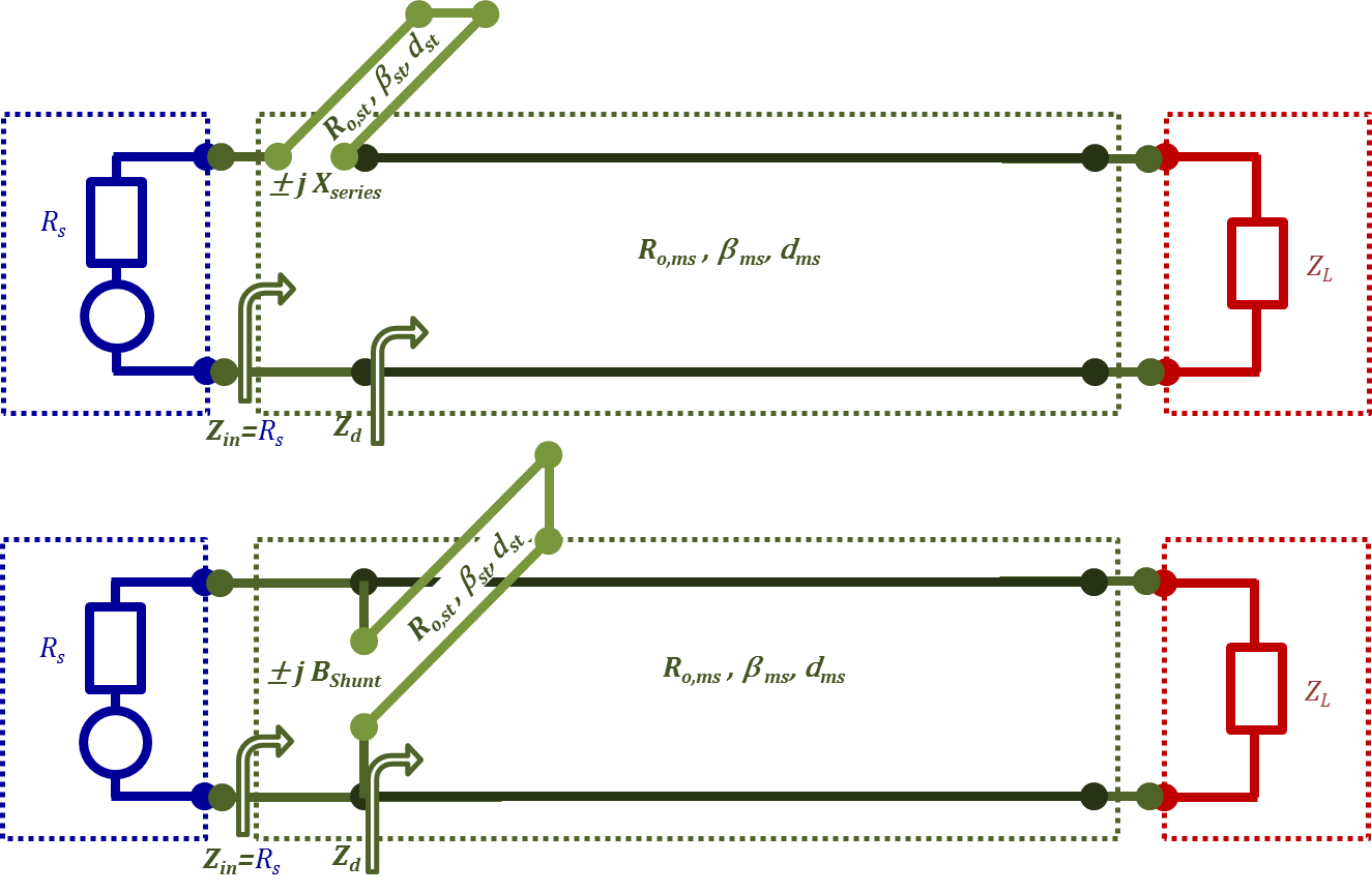
Figure 2.25
Figure 2.25
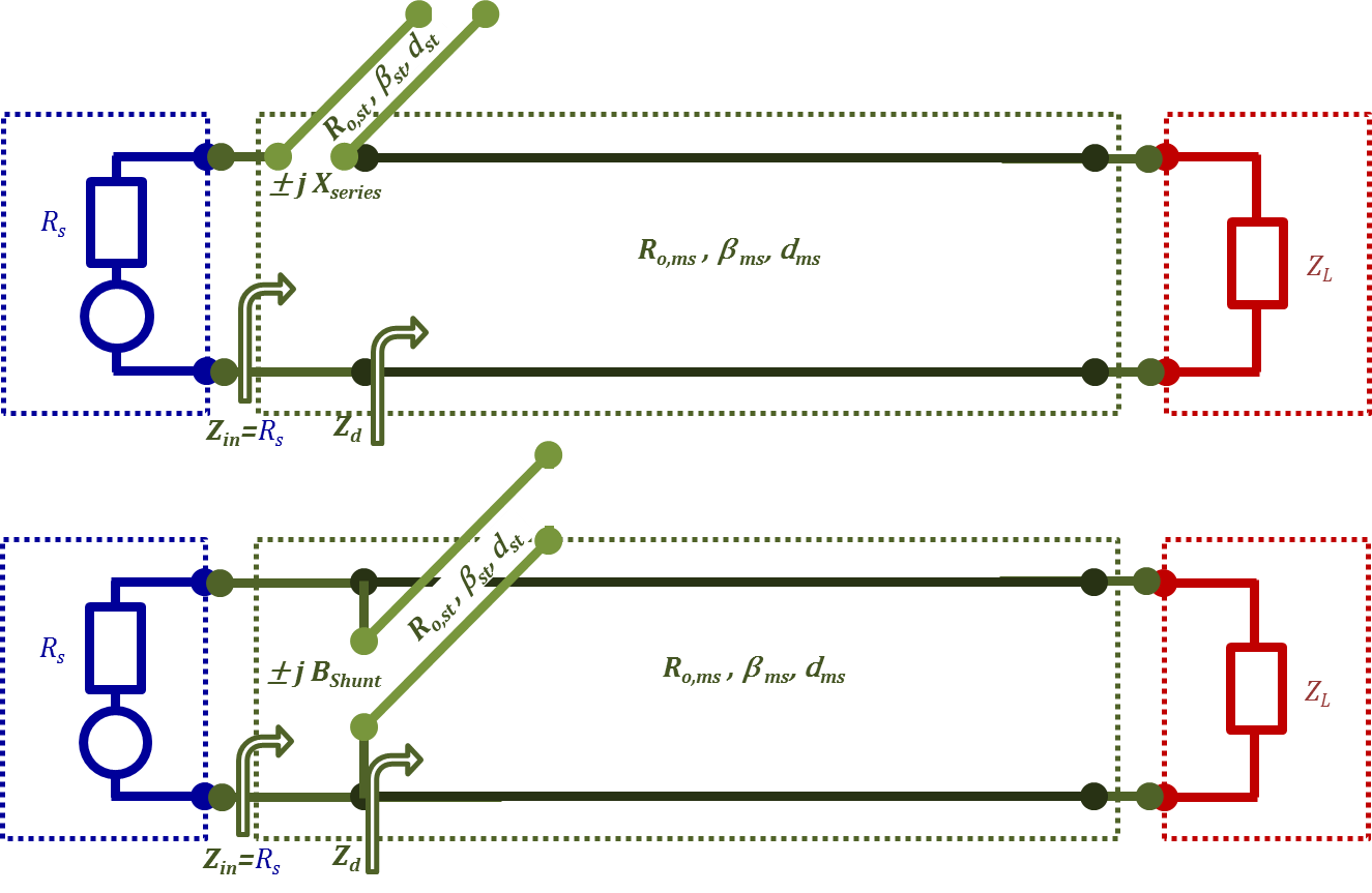
Figure 2.25
Figure 2.25b
The table below demonstrates all 8 possible single stub matching designs. In this lecture, to demonstrate the concept, we will only consider the case of short-circuited shunt stub matching presented in the lower part of Figure 2.25. This case correspond to the shaded columns in the table.
|
Short Circuited Stub |
Open Circuited Stub |
|||||||
|
Series/Shunt (Parallel) |
Series |
Shunt |
Series |
Shunt |
||||
|
Capacitive/Inductive |
Cap |
Ind |
Cap |
Ind |
Cap |
Ind |
Cap |
Ind |
|
Stub Location $d_{ms}$ |
||||||||
|
Line Impedance/Admittance at stub location |
||||||||
|
Needed stub input Impedance/Admittance (at line) |
||||||||
|
Stub Length $d_{st}$ |
||||||||
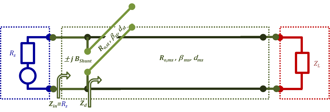
Figure 2.25c
Figure 2.25c
As you recall, the equations for this case were Equations (2.78), (2.79), and (2.81).
$ Real~part~of \left\{ {{Y}_{d}}={{\left[ {{R}_{o,ms}}\frac{\left[ {{Z}_{L}}+{{R}_{o,ms}}\cdot j~tan\left( {{\beta }_{ms}}{{d}_{ms}} \right) \right]}{\left[ {{R}_{o,ms}}~+~{{Z}_{L}}\cdot j~tan\left( {{\beta }_{ms}}{{d}_{ms}} \right) \right]} \right]}^{-1}} \right\}={{\left[ {{R}_{s}} \right]}^{-1}}\tag {2.78}$
$\pm j{{B}_{shunt}}+Imaginary~part~of\left\{ {{Y}_{d}}={{\left[ {{R}_{o,ms}}\frac{\left[ {{Z}_{L}}+{{R}_{o,ms}}\cdot j\tan \left( {{\beta }_{ms}}{{d}_{ms}} \right) \right]}{\left[ {{R}_{o,ms}}~+~{{Z}_{L}}\cdot j~tan\left( {{\beta }_{ms}}{{d}_{ms}} \right) \right]} \right]}^{-1}} \right\}=0 \tag {2.79}$
$\pm j{{B}_{shunt}}={{\left[ j~{{R}_{o,st}}\cdot \tan \left( {{\beta }_{st}}{{d}_{st}} \right) \right]}^{-1}}$
The objective is to find answers for the location of the stub on the TL, $d_{ms}$, as well as the stub length, $d_{st}$. In the following, we will demonstrate the use of the Smith chart for working out these equations.
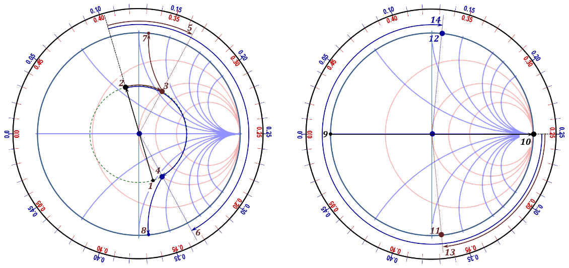
Figure 2.51
Figure 2.51
Choose the normalization impedance to be $Z_{o}$ to be matched to ($R_{s}$ in this case).
1. Compute the normalized $Z_{Ln}$ = $Z_{L}$/$Z_{o}$.
2. Locate $Z_{Ln}$ on the chart and identify the $Γ_{L}$ phasor point [1].
3. Draw a circle centered at the origin passing by $Γ_{L}$.
4. Extend the $Γ_{L}$ phasor through the origin to reach the $–Γ_{L}$ point [2]. This is the $Y_{Ln}$ point.
5. Move on the circle of step 4 above "towards generator" until it intercepts the g=1 (r=1) circle. There will be two intercept points [3] and [4]. This step is the realization of Equation (2.78) where the normalized real part of the line admittance is 1, and hence the real part of the admittance equals that of the desired matching value. Having the real part of the line admittance matched, what remains is to tune out (null) the imaginary part using the stub susceptance. Hence, the identified intercept points define the proper location for adding the shunt stub.
6. Determine the normalized distances moved from the load location to the two-intercept points: $d_{ms1}$/λ [5] and $d_{ms2}$/λ [6], respectively.
7. In principle, additional rotations of integer multiples of λ/2 will bring us to the same points, which means that we have many possible solutions in the form of {$d_{ms1}$/ λ + 0.5 n} and {$d_{ms2}$/ λ + 0.5 n}, where n is an integer. Typically, the first two intercepts are presented as the proposed stub locations.
8. Determine the line normalized susceptances for both solutions. Notice that both values are symmetrically located and thus have the same magnitude but opposite polarities, e.g. $jb_{ms1}$ [7] and $jb_{ms2}$ (-$jb_{ms1}$) [8] corresponding to the $d_{ms1}$ and $d_{ms2}$ solutions, respectively.
9. The chosen stub is needed to null the line susceptance and hence the stub susceptance should be equal but opposite in polarity to that of the line. Hence, the desired stub susceptances should be $jB_{st1}$ = -($jb_{ms1}$*$Y_{o}$) and $jB_{st2}$ = -($jb_{ms2}$*$Y_{o}$), respectively.
10. Compute the normalized stub susceptances with respect to its characteristic impedance: $jb_{st1}$ = $jB_{st1}$/$Y_{o,st}$ and $jb_{st2}$ = $jB_{st2}$/$Y_{o,st}$, respectively.
11. To determine the proper stub length(s), we need to do another chart for the stub as a TL with a zero load impedance (infinite load admittance) and known input admittance (susceptance). This chart can be done on the same chart we used for the matching section line without interfering with the first solution. This is because the circle trace of the stub line is the circle that passes by zero load impedance (infinite admittance) which is the r=0 circle (the biggest circle on the chart). If you prefer, you may use a separate chart for the stub section.
12. Locate the zero impedance load for the stub [9]. In admittance terms, the short circuited load end is on the opposite side of the chart (the point ∞,∞) [10].
13. Locate the two possible stub susceptances on the chart, $jb_{st1}$ and $jb_{st2}$, [11] and [12].
14. Starting at the (∞,∞) point and moving towards the generator, determine the normalized distances to be moved to arrive at the desired stub susceptances, $d_{st1}$ [13] and $d_{st2}$ [14], respectively.
15. Again, additional rotations of integer multiples of λ/2 yield valid answers which means that again we have many possible solutions in the form of {$d_{st1}$/ λ + 0.5 m} and {$d_{st2}$/ λ + 0.5 m}, where m is an integer. Typically, the first two solutions (m=0) are presented as the proposed stub lengths.
- What is the number of design possibilities of a short circuited matching stub?
- What are the design parameters of a matching stub?
Return to Lesson
Return to Video
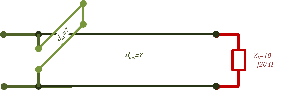
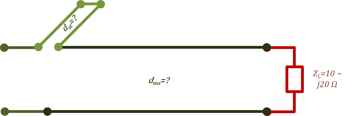
Examples II.10
- Find the design parameters of the matching stub in each of the following circuits assuming a source and TL characteristic impedances of ${50~Ohm}$each.
Return to Lesson
Return to Video
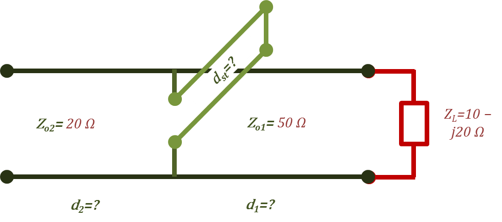
Problems II.10
- For the circuit given in the following figure, assuming a source impedance of ${20~Ohm}$, find the values of all the unknown parameters that will result in a perfect match.