Chapter II-Lesson 1 of 10 Transmission Lines - Wave Equations
Instructions
- Read the lecture (displayed below) [30-60 minutes]
- Watch the video (26:40+7:32 minutes) [35 minutes]
- Do the exercises [~30 minutes]
Total time = [~2:00 hours]
Why study TL ‐ Circuit size and frequency
Transmission Lines, TL, is the name we use to refer to those wires and cables that connect electrical and electronic devices (parts or components) to each other. The wires used to connect the light bulb to the electrical mains is a transmission line, the wire that connects the landline phone to the wall outlet is a transmission line, and the cable that connects the TV to the satellite receiver, the wall outlet, or antenna is also a transmission line. The wires you used in the circuits and electronics laboratories, and the wires you used in “bread-boarding” an analog or a digital circuit are all transmission lines. The conducting strips on (and within) the motherboard of the computer as well as the “interconnects” inside the semiconductor chips (processor, memory, etc.) are also transmission lines. Figure 2.1 demonstrates a few samples of different kinds of Transmission Lines.
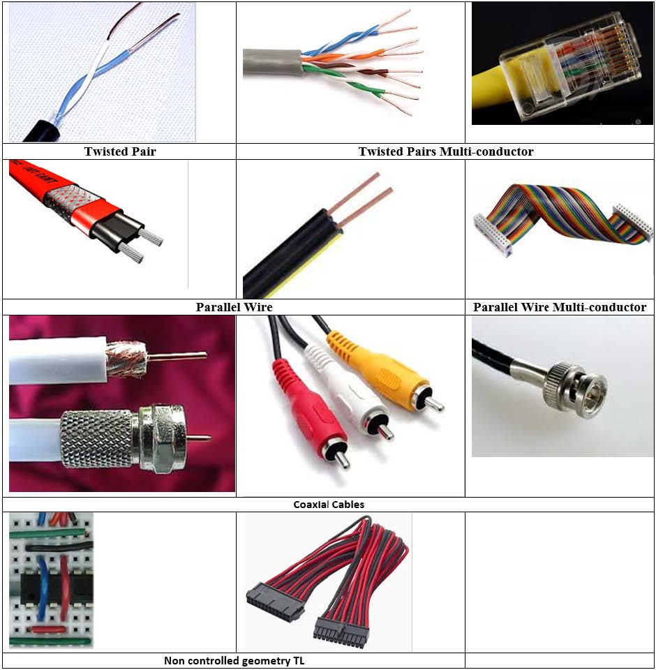
Figure 2.1 Different Kinds of Transmission Lines
Figure 2.1
“Ok. So, what is so important about transmission lines to make this topic the opening chapter of an EM book?” We used those wires in our circuits and electronics labs with no issues whatsoever. We also wired so many of these “bread-boards” and things worked well. The answer is that it has to do with the length of the wire relative to the wavelength of the signals propagating, as well as the wire’s internal resistance. Let us take these two items one at a time. First, we talk about wire length and wavelength.
To remind you about wavelength, we visualize a signal/wave propagating in one dimension, see Figure 2.2. Well, as the figure shows, the signal travels a distance as time elapses. The distance between two consecutive locations of similar phase on the wave (e.g. two consecutive peaks) is called the wavelength, λ. Simple physics tells us that that distance λ$=c/f$, where $c$ is the wave’s phase velocity and $f$ is its frequency.
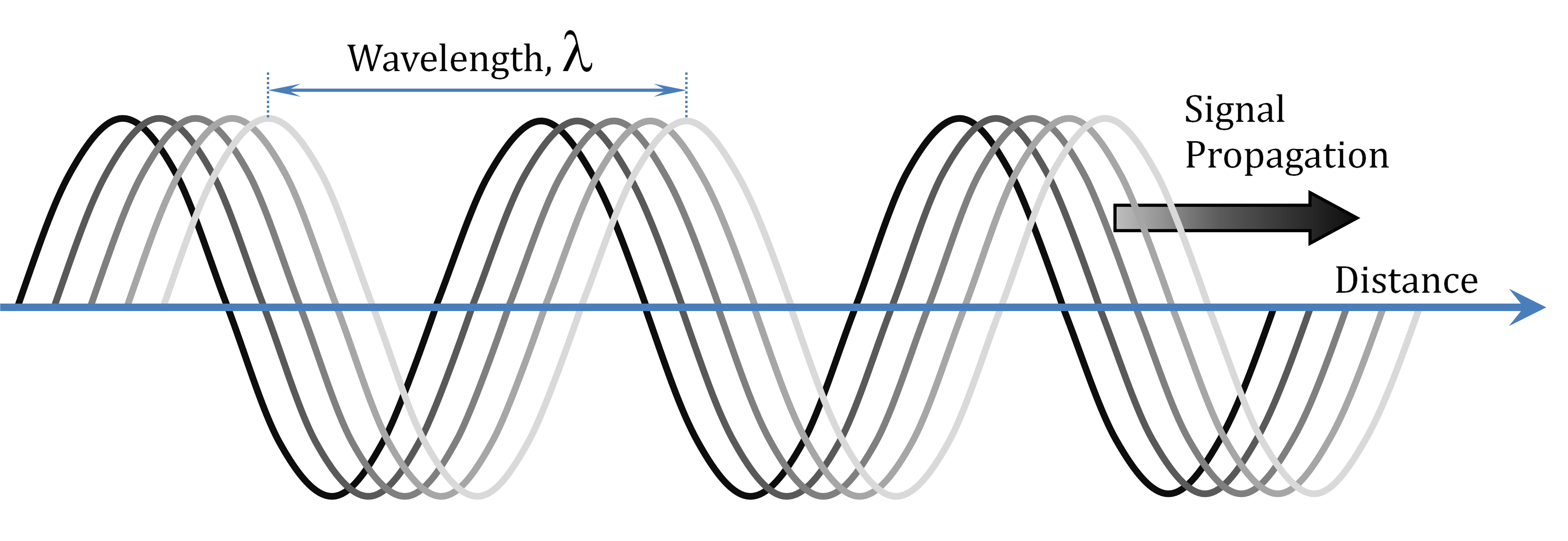
Figure 2.2
Figure 2.2
Now, let us assume that this signal propagates along a conducting wire (cable/transmission line) of length $ℓ$. Figures 2.3 demonstrates that the signal phase varies along the TL length. The amount of phase variation along the TL length, $ℓ$, depends on the length of this wire relative to the wavelength, λ. The ratio $ℓ$/λ is the same as $(Δ~phase~/360)$.
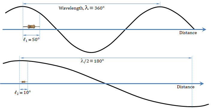
Figure 2.3
Figure 2.3
Hence, the change in signal phase between that at the beginning of the TL segment $ℓ$ and its end, $Δ$ phase, equals $360*ℓ$/λ. This change in phase corresponds to a change in signal amplitude (see the figure), and hence the signal at the beginning of the TL segment $ℓ$ and its end are not identical. Consequently, if you are using this line to connect the output side of a device or a component and the input of another, then, one cannot assume that the signal that came out the first device entered into the second. Rather one should account for the changes introduced by the interconnecting TL.
Working at low frequencies, the wavelength is long and most typical wiring arrangements are too short compared to it. In these cases, the $Δ$ phase is infinitesimally small and so is the change in signal amplitude. [Notice that for DC “signals” (zero frequency), the wavelength is infinite]
Now, we turn briefly to the second item, “the wire’s internal resistance” which may not be ignored even if $ℓ$/λ is infinitesimally small. At low frequencies and at DC, we would only be concerned about the signal drop as a result of the wire’s internal resistance.
Back to the cases where the ratio $ℓ$/λ matters. The question is how much $ℓ$/λ can we tolerate (ignore) in our analysis (design)? The answer to this question lies in deciding how much signal level (and hence phase) change can be tolerated. Considering the wave changes the fastest around its zero crossing where $sin\left(x\right)≈x$, then the worst-case analysis holds. Table 2.1 demonstrates the orders of magnitudes of circuit dimensions that can be tolerated at different operating frequencies. Three “tolerance” levels are given corresponding to different levels of phase errors.
| % Change in Signal Amplitude [x] | 10.0% |
1.0% |
0.1% |
| Corresponding $\Delta{}$ Phase in Radians [sin$^{-1}$(x)] | 0.100 |
0.010 |
0.001 |
| Corresponding $\Delta{}$ Phase in Degrees | 5.739 |
0.573 |
0.057 |
| Corresponding $ℓ$/λ [$\Delta{}$ Phase/2$\pi{}$] | 0.016 |
0.0016 |
0.00016 |
Frequency |
Wavelength in air |
Tolerated Length (air) |
Tolerated Length (air) |
Tolerated Length (air) |
Metric Unit |
1 Hz |
300.0 |
4.78264 |
0.47747 |
0.04775 |
Mm |
60 Hz |
5.0 |
0.07971 |
0.00796 |
0.00080 |
Mm |
1 kHz |
300.0 |
4.78264 |
0.47747 |
0.04775 |
Km |
1 MHz |
300.0 |
4.78264 |
0.47747 |
0.04775 |
M |
10 MHz |
30.0 |
0.47826 |
0.04775 |
0.00477 |
M |
100 Mhz |
3.0 |
0.04783 |
0.00477 |
0.00048 |
M |
1 GHz |
30.0 |
4.78264 |
0.47747 |
0.04775 |
mm |
10 GHz |
3.0 |
0.47826 |
0.04775 |
0.00477 |
mm |
100 GHz |
3.0 |
0.04783 |
0.00477 |
0.000477 |
mm |
1 THz |
0.3 |
4.78264 |
0.47747 |
0.04775 |
µm |
Frequency |
wavelength |
Tolerated Length (air) |
Tolerated Length (air) |
Tolerated Length (air) |
English Unit |
1 Hz |
186,411 |
2,971.79600 |
296.68784 |
29.66829 |
mile |
60 Hz |
3,107 |
49.52993 |
4.94480 |
0.49447 |
mile |
1 kHz |
186 |
2.97180 |
0.29669 |
0.02967 |
mile |
1 MHz |
0.186 |
0.00297 |
0.00030 |
0.00003 |
mile |
10 MHz |
98.4 |
1.56911 |
0.15665 |
0.01566 |
feet |
100 Mhz |
9.84 |
0.15691 |
0.01567 |
0.00157 |
foot |
1 GHz |
11.8 |
0.18829 |
0.01880 |
0.00188 |
inch |
10 GHz |
1.18 |
0.01883 |
0.00188 |
0.000188 |
inch |
100 GHz |
0.118 |
1.8829 |
0. 18829 |
0.018829 |
mil |
1 THz |
0.0118 |
0. 18829 |
0.018829 |
0.0018829 |
mil |
So, as you can see, if you are building a circuit (or device) to operate at 1 GHz, your wiring interconnects should be shorter than 0.04775 cm (0.0188”), otherwise you must analyze the performance of such interconnect using “Transmission Line Theory” to avoid errors more than 1%.
Transmission Line Analysis (Theory)
The accurate and comprehensive way to analyze the performance of transmission lines is to do the analysis as an electromagnetic fields problem. This requires the use of Maxwell’s equations to develop a full EM field model and study the field waves as they propagate along the TL. This process will be the subject of Chapter XIII of this book. This means that there is a lot for us to learn before we can get into such analysis. However, we can use a circuit theory approach to develop a circuit model and get a simplified analysis for the TL for the time being.
The interesting point here is that the circuit theory tools that we will be using to develop TL analysis are not but the derivatives of the field theory and Maxwell’s equations. We learned these tools in earlier circuit courses and we are familiar with them; specifically, Ohm’s Law and Kirchhoff’s Voltage and Current Laws.
Representing a TL by an equivalent circuit containing circuit elements that physically models the TL requires future knowledge that will be developed in later chapters as well. However, let us assume that we guess what these circuit elements are like (qualitatively) and have some physical insight of their nature. For example, we can guess that the line conductors do have some internal resistance $(R)$, the TL as a “loop” of two conductors has magnetic “inductive” behavior $(L)$, the two conductors separated by a dielectric represent a capacitance $(C)$, and the imperfect dielectric isolation between the two conductors would cause leakage “conduction” $(G)$. While we are familiar with these components in circuit analysis, the EM field definition and physical insight of these components will be the subject of later chapters in this book (Capacitance, Chapter VI – Inductance, Chapter IX, and resistance and Conductance, Chapter VI).
Circuit Theory Analysis of a Two Conductor Controlled Geometry TL
In this book, we will confine our study of TL theory to the simplest of cases; that of two conductors with uniform cross section (material and geometry do not vary along the TL length). This is what we call controlled geometry two conductor transmission line. The lines will be assumed straight with no curves or bends.
We will further limit ourselves to the case where the TL material, i.e. both conductors and the insulating dielectric(s), are linear (properties do not change with field intensity), and frequency independent (properties do not change with frequency).
Examples of such TLs include the parallel wire TL, the coaxial TL, and the microstrip TL, see Figure 2.4.
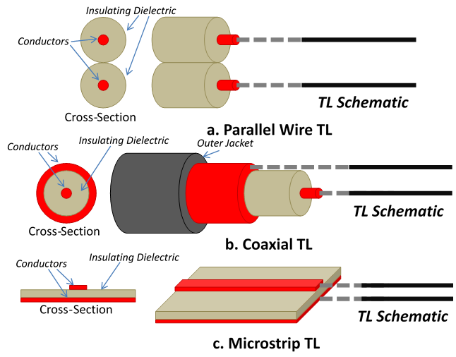
Figure 2.4 Examples of Controlled Geometry TL
Figure 2.4: Examples of Controlled Geometry TL
RLCG Model
To develop a physically based model, we have to realize that it is a distributed one, i.e. it is distributed over the length of the line and is not lumped at any specific location. To explain, we talk about the internal resistance of the two conductors forming the line. That resistance is determined by the conductor material, the cross-sectional area of the conductor, and the length of the wire. The resistance is distributed along the length of the wire and is not lumped at either end or anywhere else. So, we can model it as a distributed resistance and we can define a measure $R_{z}$ as the resistance per unit length of the transmission line. This would be the sum of the total “circuit" resistance per unit length of both TL conductors. The units of $R_{z}$ would be Ohms/m.
Likewise, we can talk about the distributed inductance of the TL circuit. We will use $L_{z}$ to denote the inductance per unit length, Henry/meter. For the insulating dielectric(s), we model two different physical parameters; $C_{z}$ (Farads/meter) and $G_{z}$ (Siemens/meter). The capacitance per unit TL length, $C_{z}$, is the physical model of the dielectric(s) insulation between the two conductors and the conductance per unit TL length, $G_{z}$, is the physical model of the imperfect insulation of the dielectric causing leakage current through the dielectric. Figure 2.5 depicts the nature of these RLCG elements. This physically based circuit model of the TL is not perfect or accurate, but it will help us set our feet into this mysterious domain of TL theory. This circuit model is typically referred to as the “RLCG” model.
It is to be noted that most references name the distributed RLCG parameters as $R$, $L$, $C$, and $G$ with no subscript. This practice may lead to some confusion as it implies a reference to “whole” resistance, inductance, capacitance and conductance quantities and not the per unit length parameters. We choose to add the $z$ subscript to distinguish these quantities as per unit $z$ length parameters. Hence, the incremental “whole” resistance of a line increment of length $Δz$ would be $ΔR=[R_{z}][Δz]$. Likewize, $ΔL=[L_{z}][Δz]$, $ΔC=[C_{z}][Δz]$, and $ΔG=[G_{z}][Δz]$ for the inremental “whole” inductance, capacitance, and conductance, respectively.
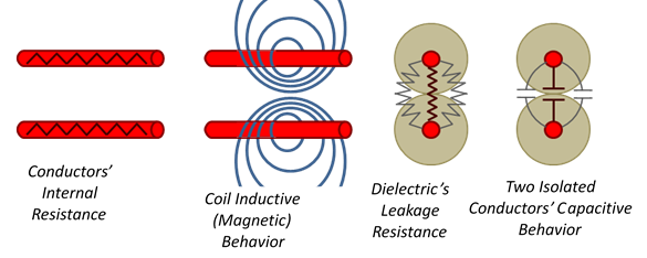
Figure 2.5
Figure 2.5
Transmission Line Circuit Analysis Using the Distributed RLCG Model
For this analysis, we will assume the line to extend along a linear axis, let us call it the $z$-axis, Figure 2.6. At $z=0$ we would have the input side (or the sending/transmitter end) to the TL (typically, a signal source with an internal “impedance”) and at the end of the line, say $z=ℓ$, the line output side, a load would be connected (receiving/receiver end).
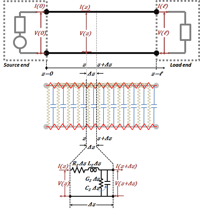
Figure 2.6
Figure 2.6
Now, as we replace the line by its distributed RLCG circuit equivalency, we expect the voltage and currents to vary with position along the line. We will use the notation $V(z)$ and $I(z)$, for the voltage and current phasors as functions position, respectively, [or $v\left( z,t \right)\text{ }\!\!~\!\!\text{ and }\!\!~\!\!\text{ }i\left( z,t \right)$ for instantaneous (time domain) expressions]. We use the upper case notations for the phasors in the frequency domain analysis, while the lower case represent the time domain variables. At $z$ = 0 and at $z$ = $ℓ$, the voltage and current terms would be $V(0)$, $I(0)$, $V(ℓ)$, and $I(ℓ)$, [or $v\left( 0,t \right),~i\left( 0,t \right),~v\left( ℓ,t \right),$ and $i\left( ℓ,\text{t} \right)]$, respectively.
Next, we need to develop expressions for the voltages current relationships as functions of position and time. In order to develop a thorough and insightful analysis of the TL network, we intend to carry the analysis in both the time and frequency domains simultaneously. Moreover, we will also be monitoring the solutions for both the transient and the steady (harmonic analysis) states as we go. As we take the analysis back and forth between the two domains, some readers may find it a bit confusing. However, going over this section a couple of times, and with focused attention, the results will be all positive.
Steady-State Harmonic Analysis
In the following, we will start with the steady-state harmonic analysis in both time and frequency domains. We will assume an excitation in the form of a time harmonic voltage
${{v_s}}\left( t \right)=\left| {{V_s}} \right|\cos \left( \omega t+{{\varphi s}} \right)~~~[time~ dom] \Leftrightarrow [freq~ dom]~~~{{V_s}}\left( j\omega \right)=\left| {{V_s}} \right|{{e}^{j{{\varphi s}}}}$
Since we are limiting our discussion to a linear system (without any nonlinear elements), then all solution voltages and currents are expected to be of the same frequency as that of the source; for example, the voltage on the line at a general location $z$ at time $t$ would assume the following form:
$v\left( z,t \right)=\left| V\left( z \right) \right|\cos \left( \omega t+\varphi \left( z \right) \right)~~~[time~ dom] \Leftrightarrow [freq~ dom]~~~V\left( z,j\omega \right)=\left| V\left( z \right) \right|{{e}^{j\varphi \left( z \right)}}$
In the following, we will develop TL equations and solutions in both frequency and time domains side by side. The left column would be for the time domain development while the right one will be for the frequency domain. In doing so, we are attempting not to get “disoriented/lost in the ocean of the frequency domain and lose our ability to get back to shore”. Instead, we will constantly relate to the physics of the development and the solution by “swimming close to shore” and monitoring the time domain phenomena while doing the frequency domain development.
To analyze the "electric circuit" shown, we need to build the distributed equation for $V(z,j\omega )$ and $I(z,j\omega )$ [or $v\left( z,t \right)~and~i\left( z,t \right)$] along the line. We do that by considering an infinitesimally small increment of the line length $𝛥z$ (to start at $z$ and end at $z$+$𝛥z$). Writing the circuit (input-output) relationships between the voltages and currents for the $𝛥z$ increment enables us to build the differential equation describing the behavior of this physically based circuit model. To do that, we use Kirchhoff's Voltage and Kirchhoff's Current Laws (KVL and KCL) for the $𝛥z$ "equivalent" circuit (see Figure 2.6).
Time Domain Analysis: $v\left( z,t \right)~and~i\left( z,t \right)$ |
Eq # |
Frequency Domain Analysis: $V\left( z,j\omega \right)~and~I\left( z,j\omega \right)$ |
Forming the Differential Equations: |
||
We start with the differential relationship, while skipping the writing of $'',t''$and $''j\omega ''$” in all voltage and current expressions |
||
$v\left( z+Δz,t \right)=v\left( z,t \right)+Δv\left( z,t \right)$ |
(2.1) |
$V\left( z+Δz \right)=V\left( z \right)+ΔV\left( z \right)$ |
$i\left( z+Δz,t \right)=i\left( z,t \right)+Δi(z,t)$ |
(2.2) |
$I\left( z+Δz \right)=I\left( z \right)+ΔI(z)$ |
Now, we apply KVL |
||
$v\left( z,t \right)={{v_R}}+{{v_L}}+\left[ v\left( z+Δz,t \right) \right]$ |
(2.3) |
$V\left( z \right)={{V_R}}+{{V_L}}+\left[ V\left( z+Δz \right) \right]$ |
Where ${{v_R}}~and~{{v_L}}$ $[{{V_R}}~and~{{V_L}}]$ are the voltage drops across ${{Rs}}Δz$ and ${{Ls}}Δz$, and using line (2.1) |
||
$v\left( z,t \right)=\left( {{R}_{z}}~Δz \right)\cdot i\left( z,t \right)+\left( {{L}_{z}}~Δz \right)\cdot \frac{di\left( z,t \right)}{dt}+\left[ v\left( z,t \right)+Δv\left( z,t \right) \right]$ |
(2.4) |
$V\left( z \right)=\left( {{R}_{z}}~Δz \right)\cdot I\left( z \right)+\left( j\omega {{L}_{z}}~Δz \right)\cdot I\left( z \right)+\left[ V\left( z \right)+ΔV\left( z \right) \right]$ |
$\frac{Δv\left( z,t \right)}{Δz}=-\left\{ {{R}_{z}}\cdot i\left( z,t \right)+{{L}_{z}}\cdot \frac{di\left( z,t \right)}{dt} \right\}$ |
(2.5) |
$\frac{ΔV\left( z \right)}{Δz}=-\left\{ {{R}_{z}}\cdot I\left( z \right)+j\omega {{L}_{z}}\cdot I\left( z \right) \right\}$ |
Taking the limit as $Δz$ becomes infinitesimally small and approaches zero |
||
$\frac{dv\left( z,t \right)}{dz}=-\left\{ {{R}_{z}}\cdot i\left( z,t \right)+{{L}_{z}}\cdot \frac{di\left( z,t \right)}{dt} \right\}$ |
(2.6) |
$\frac{dV\left( z \right)}{dz}=-\left\{ {{R}_{z}}+j\omega {{L}_{z}} \right\}\cdot I\left( z \right)$ |
Next, we apply KCL |
||
$i\left( z,t \right)={{i_G}}+{{i_C}}+\left[ i\left( z+Δ\,z,t \right) \right]$ |
(2.7) |
$I\left( z \right)={{I_G}}+{{I_C}}+\left[ I\left( z+Δz \right) \right]$ |
Where ${{i_G}}~and~{{i_C}}$ $\left[ {{I_G}}~and~{{I_C}} \right]$ are the current drops through ${{G}_{z}}Δz$ and ${{C}_{z}}Δz$, and using Equation (2.2) |
||
$i\left( z,t \right)=\left( {{G}_{z}}Δz \right)\cdot v\left( z+Δz,t \right)+\left( {{C}_{z}}Δz \right)\cdot \frac{dv\left( z+Δz,t \right)}{dt}+\left[ i\left( z,t \right)+Δi\left( z,t \right) \right]$ |
(2.8) |
$I\left( z \right)=\left( {{G}_{z}}Δz \right)\cdot V\left( z+Δz \right)+\left( j\omega \,{{C}_{z}}Δz \right)\cdot V\left( z \right)+ \\~~~~~~~~~~~~~ \left[ I\left( z \right)+ΔI\left( z \right) \right]$ |
$\frac{Δi\left( z,t \right)}{Δz}=-\left\{ {{G}_{z}}\cdot v\left( z+Δz,t \right)+{{C}_{z}}\cdot \frac{dv\left( z+Δz,t \right)}{dt} \right\}$ |
(2.9) |
$\frac{ΔI\left( z \right)}{Δz}=-\left\{ {{G}_{z}}\cdot V\left( z+Δz \right)+j\omega \,{{C}_{z}}\cdot V\left( z+Δz \right) \right\}$ |
Taking the limit as $Δz$becomes infinitesimally small and approaches zero |
||
$\frac{di\left( z,t \right)}{dz}=-\left\{ {{G}_{z}}\cdot v\left( z,t \right)+{{C}_{z}}\cdot \frac{dv\left( z,t \right)}{dt} \right\}$ |
(2.10) |
$\frac{dI\left( z \right)}{dz}=-\left\{ {{G}_{z}}+j\omega \,{{C}_{z}} \right\}\cdot V\left( z \right)$ |
Solution: |
||
We have two simultaneous differential equations in $i~and~v$. So, we need to combine them in a way to end up with a new equation in one variable only. |
||
Differentiate line (2.6) with respect to (z) and line (2.10) with respect to (t) |
|
Differentiate line (2.6) with respect to z and using line (2.10) |
$\frac{{{d}^{2}}v\left( z,t \right)}{d{{z}^{2}}}=-\left\{ {{R}_{z}}\cdot \frac{di\left( z,t \right)}{dz}+{{L}_{z}}\cdot \frac{{{d}^{2}}i\left( z,t \right)}{dtdz} \right\}$ |
(2.11) |
$\frac{{{d}^{2}}V\left( z \right)}{d{{z}^{2}}}=-\left\{ {{R}_{z}}+j\omega {{L}_{z}} \right\}\cdot \frac{dI\left( z \right)}{dz}$ |
$\frac{{{d}^{2}}i\left( z,t \right)}{dzdt}=-\left\{ {{G}_{z}}\cdot \frac{dv\left( z,t \right)}{dt}+{{C}_{z}}\cdot \frac{{{d}^{2}}v\left( z,t \right)}{d{{t}^{2}}} \right\}$ |
(2.12) |
|
Combining lines (2.11) and (2.12) |
|
Combining lines (2.10) and (2.11) |
$\frac{{{d}^{2}}v\left( z,t \right)}{d{{z}^{2}}}=-\left\{ {{R}_{z}}\cdot \left( -\left\{ {{G}_{z}}\cdot v\left( z,t \right)+{{C}_{z}}\cdot \frac{dv\left( z,t \right)}{dt} \right\} \right)+ \\~~~~~~~~~~~~~ {{L}_{z}}\cdot \left( -\left\{ {{G}_{z}}\cdot \frac{dv\left( z,t \right)}{dt}+{{C}_{z}}\cdot \frac{{{d}^{2}}v\left( z,t \right)}{d{{t}^{2}}} \right\} \right) \right\}$ |
(2.13) |
|
$\frac{{{d}^{2}}v\left( z,t \right)}{d{{z}^{2}}}=\left\{ {{R}_{z}}{{G}_{z}}\cdot v\left( z,t \right)+\left[ {{R}_{z}}{{C}_{z}}+{{L}_{z}}{{G}_{z}} \right]\cdot \frac{dv\left( z,t \right)}{dt}+{{L}_{z}}{{C}_{z}}\cdot \frac{{{d}^{2}}v\left( z,t \right)}{d{{t}^{2}}} \right\}$ |
(2.14) |
$\frac{{{d}^{2}}V\left( z \right)}{d{{z}^{2}}}=\left\{ {{R}_{z}}+j\omega {{L}_{z}} \right\}\cdot \left\{ {{G}_{z}}+j\omega {{C}_{z}} \right\}\cdot V\left( z \right)$ |
Hence, here we have one equation in one variable; the voltage. It is important to recognize that the resulting Equation (2.14) is a second order differential equation, D.E. We combined two first order D.E. to yield one second order one. |
||
To solve the D.E. in (2.14), we use the Laplace Transform |
|
|
$\frac{{{d}^{2}}V\left( z \right)}{d{{z}^{2}}}=\left\{ {{R}_{z}}{{G}_{z}}\cdot V\left( z \right)+\left[ {{R}_{z}}{{C}_{z}}+{{L}_{z}}{{G}_{z}} \right]\cdot sV\left( z \right)+{{L}_{z}}{{C}_{z}}\cdot {{s}^{2}}V\left( z \right) \right\}$ |
|
|
$\frac{{{d}^{2}}V\left( z,s \right)}{d{{z}^{2}}}=\left\{ {{R}_{z}}+s{{L}_{z}} \right\}\cdot \left\{ {{G}_{z}}+s{{C}_{z}} \right\}\cdot V\left( z \right)$ |
(2.15) |
$\frac{{{d}^{2}}V\left( z,j\omega \right)}{d{{z}^{2}}}=\left\{ {{R}_{z}}+j\omega {{L}_{z}} \right\}\cdot \left\{ {{G}_{z}}+j\omega {{C}_{z}} \right\}\cdot V\left( z \right)$ |
Defining ${{\gamma }^{2}}$ |
||
${{\gamma }^{2}}\left( s \right)=~{{R}_{z}}{{G}_{z}}+s\left[ {{R}_{z}}{{C}_{z}}+{{L}_{z}}{{G}_{z}} \right]+{{s}^{2}}{{L}_{z}}{{C}_{z}}$ |
(2.16) |
${{\gamma }^{2}}\left( j\omega \right)=\left\{ {{R}_{z}}+j\omega {{L}_{z}} \right\}\cdot \left\{ {{G}_{z}}+j\omega {{C}_{z}} \right\}$ |
$\frac{{{d}^{2}}V\left( z \right)}{d{{z}^{2}}}={{\gamma }^{2}}\cdot V\left( z \right)$ |
(2.17) |
$\frac{{{d}^{2}}V\left( z \right)}{d{{z}^{2}}}={{\gamma }^{2}}\cdot V\left( z \right)$ |
Solving the DE in line (2.17) |
||
$V\left( z \right)={{V}^{+}}{{e}^{-\gamma z}}+{{V}^{-}}{{e}^{+\gamma z}}$ |
(2.18) |
$V\left( z \right)={{V}^{+}}{{e}^{-\gamma z}}+{{V}^{-}}{{e}^{+\gamma z}}$ |
$Where~{{V}^{+}}and~{{V}^{-}}~are~constants$ |
||
Laplace Transform applied to line 6 |
|
From line 6 |
$\frac{dV\left( z \right)}{dz}=-\left\{ {{R}_{z}}+s{{L}_{z}} \right\}\cdot I\left( z \right)$ |
(2.19) |
|
$I\left( z \right)=-\frac{1}{\left\{ {{R}_{z}}+s{{L}_{z}} \right\}}\cdot \frac{dV\left( z \right)}{dz}$ |
(2.20) |
$I\left( z \right)=-\frac{1}{\left\{ {{R}_{z}}+j\omega {{L}_{z}} \right\}}\cdot \frac{dV\left( z \right)}{dz}$ |
$I\left( z \right)=\frac{\gamma }{\left\{ {{R}_{z}}+s{{L}_{z}} \right\}}\cdot \left\{ {{V}^{+}}{{e}^{-\gamma z}}-{{V}^{-}}{{e}^{+\gamma z}} \right\}$ |
(2.21) |
$I\left( z \right)=\frac{\gamma }{\left\{ {{R}_{z}}+j\omega {{L}_{z}} \right\}}\cdot \left\{ {{V}^{+}}{{e}^{-\gamma z}}-{{V}^{-}}{{e}^{+\gamma z}} \right\}$ |
$\frac{\gamma }{\left\{ {{R}_{z}}+s{{L}_{z}} \right\}}=~\frac{1}{{{Z}_{o}}}$ |
(2.22) |
$\frac{\gamma }{\left\{ {{R}_{z}}+j\omega {{L}_{z}} \right\}}=~\frac{1}{{{Z}_{o}}}$ |
Discussion of Possible Solutions: |
|
Summary: |
The inverse Laplace transform of these equations back to the time domain in the general case is too complicated. However, possible solutions can be achieved for either the case of harmonic signals $\left( s=j\omega \right)$ and the case of lossless TL $({{R}_{z}}=0~and~{{G}_{z}}=0)$ |
(2.23) |
$I\left( z \right)=~\frac{1}{{{Z}_{o}}}\cdot \left\{ {{V}^{+}}{{e}^{-\gamma z}}-{{V}^{-}}{{e}^{+\gamma z}} \right\}$ |
(2.24) |
${{Z}_{o}}={{Ro}}+j{{Xo}}=\sqrt{\left\{ {{R}_{z}}+j\omega {{L}_{z}} \right\}/\left\{ {{G}_{z}}+j\omega {{C}_{z}} \right\}}$ |
|
(2.25) |
$\gamma =\alpha +j\beta =\sqrt{\left\{ {{R}_{z}}+j\omega {{L}_{z}} \right\}\cdot \left\{ {{G}_{z}}+j\omega {{C}_{z}} \right\}}$ |
|
|
(2.26) |
$V\left( z \right)={{V}^{+}}{{e}^{-\gamma z}}+{{V}^{-}}{{e}^{+\gamma z}}$ |
Case of steady state harmonic signals $\left( s=j\omega \right)$: See Right Column starting line (2.23) |
(2.27) |
$V\left( z \right)={{V}^{+}}{{e}^{-\alpha z}}{{e}^{-j\beta z}}+{{V}^{-}}{{e}^{+\alpha z}}{{e}^{+j\beta z}}$ |
(2.28) |
Transfer Back to Time Domain: |
|
(2.29) |
$v\left( z,t \right)=\left| {{V}^{+}} \right|{{e}^{-\alpha z}}cos\left( \omega t-\beta z+\varphi _{v}^{+} \right)+ \\ ~~~~~~~~~~~~~~~~ \left| {{V}^{-}} \right|{{e}^{+\alpha z}}cos\left( \omega t+\beta z+\varphi _{v}^{-} \right)$ |
|
|
(2.30) |
$i\left( z,t \right)=\left| {{V}^{+}}/{{Z}_{o}} \right|{{e}^{-\alpha z}}\cos \left( \omega t-\beta z+\varphi _{v}^{+}-{{\varphi z}} \right)- \\ ~~~~~~~~~~~~~~~ \left| {{V}^{-}}/{{Z}_{o}} \right|{{e}^{+\alpha z}}cos\left( \omega t+\beta z+\varphi _{v}^{-}-{{\varphi z}} \right)$ |
Case of lossless TL $({{R}_{z}}=0~\ and\ ~{{G}_{z}}=0)$ |
||
Lines (2.16) and (2.22) reduce to |
|
Lines (2.25) and (2.22) reduce to. |
${{\gamma }^{2}}\left( s \right)={{s}^{2}}{{L}_{z}}{{C}_{z}}\quad and\quad {{Z}_{o}}=\sqrt{{{L}_{z}}/{{C}_{z}}}$ |
(2.31) |
$\gamma =j\beta =j\omega \sqrt{{{L}_{z}}{{C}_{z}}}\quad and\quad {{Z}_{o}}=\sqrt{{{L}_{z}}/{{C}_{z}}}$ |
Which reduces (2.18) and (2.21) to |
|
Which reduces (2.27) and (2.23) to |
$V\left( z \right)={{V}^{+}}{{e}^{-s\sqrt{{{L}_{z}}{{C}_{z}}}z}}+{{V}^{-}}{{e}^{+s\sqrt{{{L}_{z}}{{C}_{z}}}z}}$ |
(2.32) |
$V\left( z \right)={{V}^{+}}{{e}^{-j\beta z}}+{{V}^{-}}{{e}^{+j\beta z}}$ |
$I\left( z \right)=\frac{1}{\left\{ \sqrt{{{L}_{z}}/{{C}_{z}}} \right\}}\cdot \left\{ {{V}^{+}}{{e}^{-s\sqrt{{{L}_{z}}{{C}_{z}}}z}}-{{V}^{-}}{{e}^{+s\sqrt{{{L}_{z}}{{C}_{z}}}z}} \right\}$ |
(2.33) |
$I\left( z \right)=\frac{1}{\sqrt{{{L}_{z}}/{{C}_{z}}}}\cdot \left\{ {{V}^{+}}{{e}^{-j\beta z}}-{{V}^{-}}{{e}^{+j\beta z}} \right\}$ |
Transfer Back to Time Domain: |
|
Also, (2.29) and (2.30) reduce to |
$v\left( z,t \right)={{v}^{+}}\left( t-\sqrt{{{L}_{z}}{{C}_{z}}}z \right)+{{v}^{-}}\left( t+\sqrt{{{L}_{z}}{{C}_{z}}}z \right)$ |
(2.34) |
$v\left( z,t \right)=\left| {{V}^{+}} \right|\cos \left( \omega t-\beta z+\varphi _{v}^{+} \right)+\left| {{V}^{-}} \right|~cos\left( \omega t+\beta z+\varphi _{v}^{-} \right)$ |
$i\left( z,t \right)=\frac{1}{\sqrt{{{L}_{z}}/{{C}_{z}}}}\cdot \left\{ {{v}^{+}}\left( t-\sqrt{{{L}_{z}}{{C}_{z}}}z \right)-{{v}^{-}}\left( t+\sqrt{{{L}_{z}}{{C}_{z}}}z \right) \right\}$ |
(2.35) |
$i\left( z,t \right)=\left| \frac{{{V}^{+}}}{{{Z}_{o}}} \right|\cos \left( \omega t-\beta z+\varphi _{v}^{+} \right)-\left| \frac{{{V}^{-}}}{{{Z}_{o}}} \right|~cos\left( \omega t+\beta z+\varphi _{v}^{-} \right)$ |
So, we have arrived at a solution for the steady-state harmonic case using both the time domain and the frequency domain approaches. The obtained solutions are expressed by Equations (2.29)-(2.30) in the time domain and in Equations (2.23)-(2.27) in the frequency-domain phasor format. We did not carry out the solution in the time domain; instead, we made use of the Laplace transform to solve the second order D.E. In a way, that was similar to resorting to the frequency domain for help. The Laplace domain is but a generalization of the frequency domain as it uses $s=\sigma +j\omega $ and hence allows the study of transients. When $\sigma =0$, the Laplace domain coincides with the frequency domain and the problem reduces to its steady-state harmonic solution.
In the special case of a lossless TL, we were able to carry out the solution further in the time domain to non-harmonic cases. These solutions are given by Equations (2.34)-(2.35). The corresponding harmonic solutions are given on the right hand column of the same lines.
- What is a "Transmission Line" - cite some examples?
- What is meant by "controlled geometry transmission line"?
- Why do we need to study transmission line analysis?
- For a circuit operating at ${3~GHz}$, what is the maximum size a interconnects that can be "ignored" without contributing to errors greater that ${0.1\% }$?
Return to Lesson
Return to Video
Examples II.1
- Evaluate the frequency dependent expressions for ${Z_o}$ and ${\gamma }$ for the TL with the following per unit length model parameters: ${R_z= 0.05~Ohms/m}$, ${L_z= 0.5~\mu H/m}$, ${C_z= 40~\mu F/m}$, ${G_z= 1~mS/m}$. Plot both real and imaginary parts for both ${Z_o}$ and ${\gamma }$ vs frequency for the range ${100~MHz}$ to ${10~GHz}$.
- Repeat Example 1 above for the same line neglecting the loss elements, i.e. ${R_z=0}$ and ${G_z=0}$.
Return to Lesson
Return to Video
Problems II.1
- Evaluate the Phase velocity for both exercises above - Plot vs frequency in both cases.
- Evaluate the frequency dependent expressions for ${Z_o}$ and $\gamma $ for the TL with the following per unit length model parameters: $R_z= 0.005~Ohms/m$, $L_z= 0.5~\mu H/m$, $C_z= 0.1~\mu F/m$, $G_z= 1~mS/m$. Plot both real and imaginary parts for both ${Z_o}$ and $\gamma $ vs frequency for the range $100~MHz$ to $10~GHz$.
- Evaluate the Phase velocity for problem 2 above - Plot vs frequency for the same range. Discuss the obtained result. {Hint: Heaviside distortionless Line}.
- Plot the normalized voltage (or current) time domain terms $exp (-\alpha ~z)\cdot cos (\omega ~t-\beta ~z)$ and $exp (-\alpha ~z)\cdot cos (\omega ~t+\beta ~z)$ vs $z (0-1~m)$ for the frequency $f= 1~GHz$, at time intervals of $0.1~ns$ for the duration $t=0-0.5~ns$.