Chapter III-Lesson 2 of 2 Transition to Static Electromagnetics
Instructions
- Read the lecture (displayed below) [30 minutes]
- Watch the video (TBA) [35 minutes]
- Do the exercises [~30 minutes]
Total time = [~1:00 hours]
Addendum II: Vector Calculus
Vector Definition and Examples:
A vector is a quantity characterized by having a specific magnitude and a specific direction at each point in space. In this book will use the accented notation to denote vector, e.g., a vector "F" will appear as $\vec{F}$. A vector can be expressed as a scalar multiplied by a unit vector that has the same direction as the vector itself:
$\vec{F}=F~{{\vec{a}}_{F}}$
Examples of vectors include distance, velocity, and force among many other physical quantities. The following table demonstrates some of these vector quantities.
Vector |
Examples |
| Length | 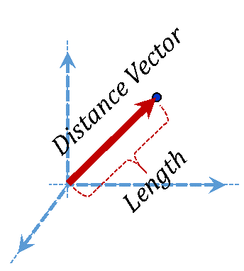 |
| Velocity | 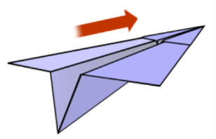 |
| Weight | 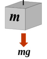 |
| Surface Area | 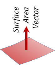 |
| Force | 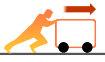 |
| Torque | 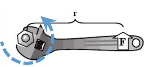 |
Vector Representations in Coordinate Systems:
To express a vector in a coordinate system is to write the vector in terms of the three orthonormal components of that coordinate system. This is done by projecting the vector along the three directions of the coordinate system and finding the magnitude of each projection. If we denote the three projections of a vector ${\vec{F}}$ along the 3 coordinates of a "1-2-3" coordinate system as F1, F2, and F3, respectively, then we can write:
${\vec{F}}={{{\vec{F}}}_{1}}+{{{\vec{F}}}_{2}}+{{{\vec{F}}}_{3}}={{{F}}_{1}}{ }~{ }{{{\vec{a}}}_{1}}+{{{F}}_{2}}{ }~{ }{{{\vec{a}}}_{2}}+{{{F}}_{3}}{ }~{ }{{{\vec{a}}}_{3}}\tag {3.1}$
where $~{{\vec{a}}_{1}},~~{{\vec{a}}_{1}},~and~~{{\vec{a}}_{1}}$ are the corresponding unit vectors of the coordinate system, Figure 3.21.
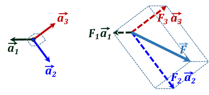
Figure 3.21
Figure 3.21
In the following, we will overview vector representation in the three coordinate systems. Two types of vectors will be demonstrated; distance vectors and others. The reason for this classification is that distance vectors are expressed in terms of the coordinate system dimensions and directions while the others will have different units but only expressed in terms of the coordinate system directions.
Vector Representation in a Cartesian coordinate system
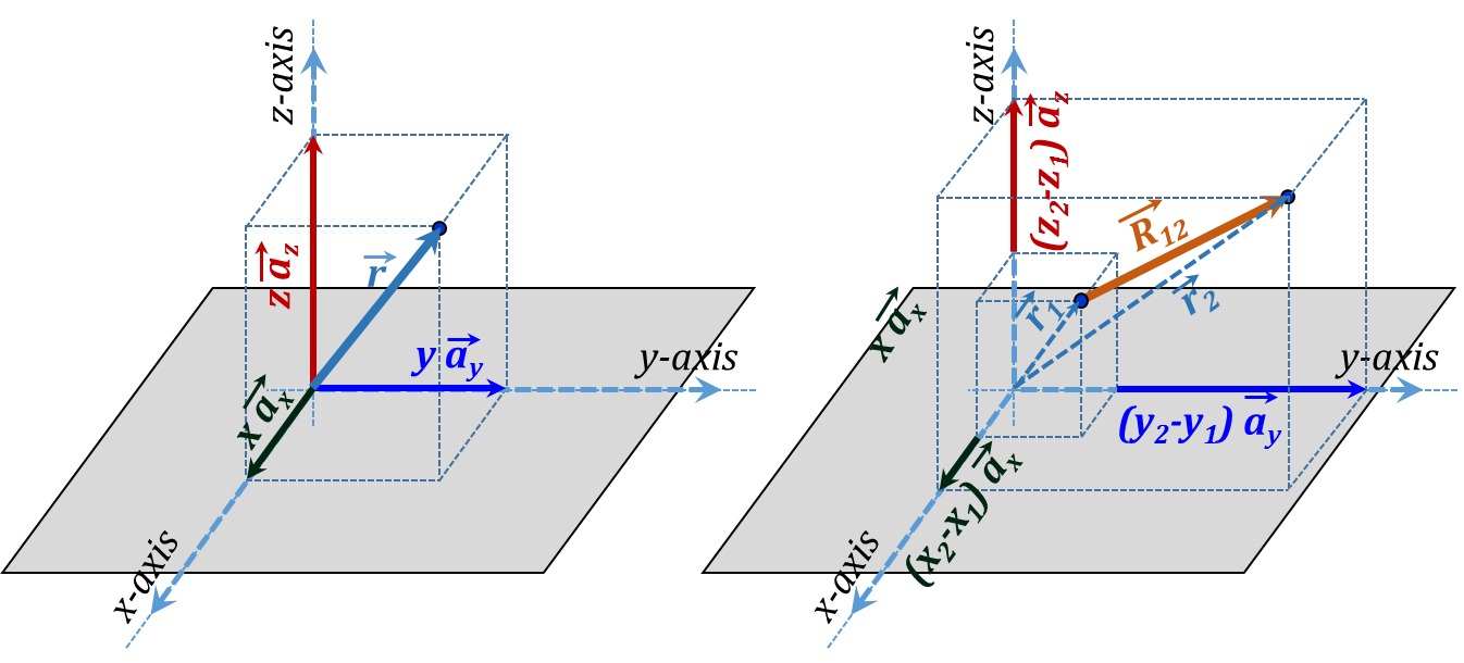
Figure 3.22
Figure 3.22
Figure 3.22 shows two types of distance vectors as represented in Cartesian coordinates; distance from the origin and distance between two points. The distance from the origin vector which we denote with the lower case r is in fact the same as the Spherical coordinate vector $\vec{r}$ which can be written as:
${\vec{r}}={x }~{ }\overrightarrow{{{{a}}_{{x}}}}+{y }~{ }\overrightarrow{{{{a}}_{{y}}}}+{z }~{ }\overrightarrow{{{{a}}_{{z}}}}\tag {3.2}$
The distance between two points (1 and 2) will be denoted by the upper case vector $\vec{R}$. This can be expressed as the difference between two $\vec{r}$ vectors as follows:
$\overrightarrow{{{{R}}_{12}}}=\overrightarrow{{{{r}}_{2}}}-{ }~{ }\overrightarrow{{{{r}}_{1}}}=\left( {{{x}}_{2}}{ }~{ }\overrightarrow{{{{a}}_{{x}}}}+{{{y}}_{2}}{ }~{ }\overrightarrow{{{{a}}_{{y}}}}+{{{z}}_{2}}{ }~{ }\overrightarrow{{{{a}}_{{z}}}} \right)-\left( {{{x}}_{1}}{ }~{ }\overrightarrow{{{{a}}_{{x}}}}+{{{y}}_{1}}{ }~{ }\overrightarrow{{{{a}}_{{y}}}}+{{{z}}_{1}}{ }~{ }\overrightarrow{{{{a}}_{{z}}}} \right)=\left( {{{x}}_{2}}-{{{x}}_{1}} \right){ }~{ }\overrightarrow{{{{a}}_{{x}}}}+\left( {{{y}}_{2}}-{{{y}}_{1}} \right){ }~{ }\overrightarrow{{{{a}}_{{y}}}}+\left( {{{z}}_{2}}-{{{z}}_{1}} \right){ }~{ }\overrightarrow{{{{a}}_{{z}}}}\tag {3.3}$
Vector representation for a general form vector
Next, we view the vector representation for a general form vector $\vec{F}$ in Cartesian coordinates. This is demonstrated in Figure 3.23 yielding the analytical expression:
${\vec{F}}={{{\vec{F}}}_{{x}}}+{{{\vec{F}}}_{{y}}}+{{{\vec{F}}}_{{z}}}={{{F}}_{{x}}}{ }~{ }{{{\vec{a}}}_{{x}}}+{{{F}}_{{y}}}{ }~{ }{{{\vec{a}}}_{{y}}}+{{{F}}_{{z}}}{ }~{ }{{{\vec{a}}}_{{z}}}\tag {3.4}$
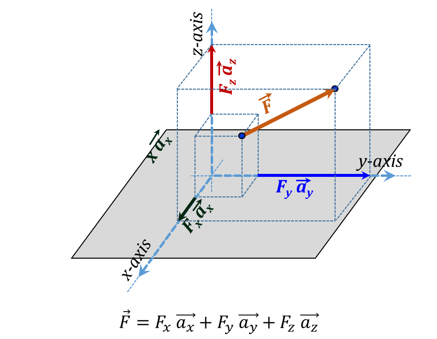
Figure 3.23
Figure 3.23
Vector Representation in Cylindrical coordinates
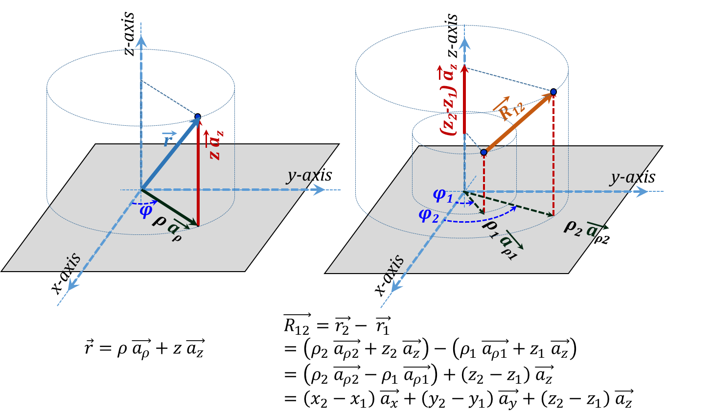
Figure 3.24
Figure 3.24
Figure 3.24 shows the two types of distance vectors as represented in Cylindrical coordinates. The distance from the origin vector $\vec{r}$ can be written as:
${\vec{r}}={ }\rho{ }~{ }\overrightarrow{{{{a}}_{{ }\rho{ }}}}+{z }~{ }\overrightarrow{{{{a}}_{{z}}}}\tag {3.5}$
It is to be noted here that the $\overrightarrow{{{a}_{\rho }}}$ unit vector is a variable one which may cause some analytical challenges in some cases especially when integration is involved. When these challenges dominate, it may be "wiser" to switch to the Cartesian coordinate representation where all the unit vectors are constants.
The distance vector$~\overrightarrow{{{R}_{12}}}$ between two points is also demonstrated in the figure. When expressed as the difference between two ${\vec{r}}$ vectors we be challenged by the vector subtraction of $\overrightarrow{{{a}_{\rho 2}}}{ }~{ }and{ }~{ }\overrightarrow{{{a}_{\rho 1}}}$:
$\overrightarrow{{{{R}}_{12}}}=\overrightarrow{{{{r}}_{2}}}-{ }~{ }\overrightarrow{{{{r}}_{1}}}=\left( {{{ }\rho{ }}_{2}}{ }~{ }\overrightarrow{{{{a}}_{{ }\rho{ }2}}}+{{{z}}_{2}}{ }~{ }\overrightarrow{{{{a}}_{{z}}}} \right)-\left( {{{ }\rho{ }}_{1}}{ }~{ }\overrightarrow{{{{a}}_{{ }\rho{ }1}}}+{{{z}}_{1}}{ }~{ }\overrightarrow{{{{a}}_{{z}}}} \right)=\left( {{{ }\rho{ }}_{2}}{ }~{ }\overrightarrow{{{{a}}_{{ }\rho{ }2}}}-{{{ }\rho{ }}_{1}}{ }~{ }\overrightarrow{{{{a}}_{{ }\rho{ }1}}} \right)+\left( {{{z}}_{2}}-{{{z}}_{1}} \right){ }~{ }\overrightarrow{{{{a}}_{{z}}}}= \\ \left( {{{x}}_{2}}-{{{x}}_{1}} \right){ }~{ }\overrightarrow{{{{a}}_{{x}}}}+\left( {{{y}}_{2}}-{{{y}}_{1}} \right){ }~{ }\overrightarrow{{{{a}}_{{y}}}}+\left( {{{z}}_{2}}-{{{z}}_{1}} \right){ }~{ }\overrightarrow{{{{a}}_{{z}}}}\tag {3.6}$
Again resorting to Cartesian coordinates offers a simple way to deal with this challenge.
Similarly, the general form vector $\vec{F}$ in Cylindrical coordinates is demonstrated in Figure 3.25. This corresponding analytical expression is:
${\vec{F}}=\overrightarrow{{{{F}}_{2}}}-{ }~{ }\overrightarrow{{{{F}}_{1}}}=\left( {{{F}}_{2{ }\rho{ }}}{ }~{ }\overrightarrow{{{{a}}_{{ }\rho{ }2}}}+{{{F}}_{2{Z }~{ }}}\overrightarrow{{{{a}}_{{z}}}} \right)-\left( {{{F}}_{1{ }\rho{ }}}{ }~{ }\overrightarrow{{{{a}}_{{ }\rho{ }1}}}+{{{F}}_{1{Z }~{ }}}\overrightarrow{{{{a}}_{{z}}}} \right)=\left( {{{F}}_{2{ }\rho{ }}}{ }~{ }\overrightarrow{{{{a}}_{{ }\rho{ }2}}}-{{{F}}_{1{ }\rho{ }}}{ }~{ }\overrightarrow{{{{a}}_{{ }\rho{ }1}}} \right)+\left( {{{F}}_{2{Z}}}-{{{F}}_{1{Z}}} \right){ }~{ }\overrightarrow{{{{a}}_{{z}}}}={{{F}}_{{x}}}{ }~{ }\overrightarrow{{{{a}}_{{x}}}}+{{{F}}_{{y}}}{ }~{ }\overrightarrow{{{{a}}_{{y}}}}+{{{F}}_{{z}}}{ }~{ }\overrightarrow{{{{a}}_{{z}}}} \tag {3.7}$
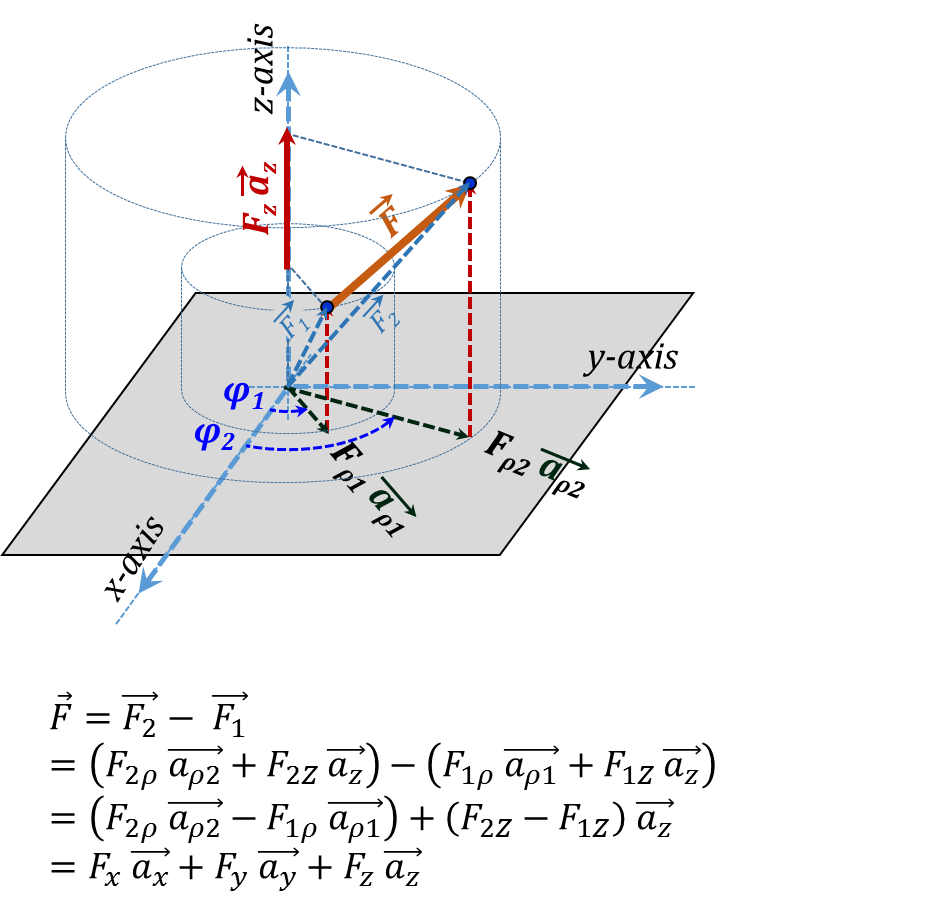
Figure 3.25
Figure 3.25
Vector Representation in Spherical coordinates
The case of Spherical coordinates, Figure 3.26, has challenges similar to those discussed in Cylindrical coordinate representation; all 3 unit vectors are variables. Switching to Cartesian offers the same convenience as discussed above.
${\vec{F}}=\overrightarrow{{{{F}}_{2}}}-{ }~{ }\overrightarrow{{{{F}}_{1}}}={{{F}}_{{x}}}{ }~{ }\overrightarrow{{{{a}}_{{x}}}}+{{{F}}_{{y}}}{ }~{ }\overrightarrow{{{{a}}_{{y}}}}+{{{F}}_{{z}}}{ }~{ }\overrightarrow{{{{a}}_{{z}}}} \tag {3.8}$
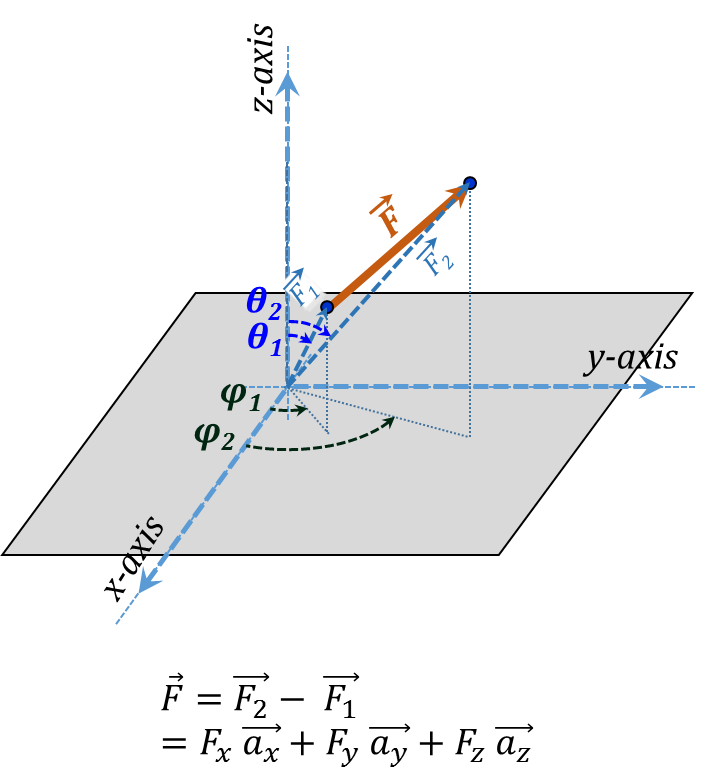
Figure 3.26
Figure 3.26
Vector Operations
The following table reviews various vector operations, gives examples of their graphical and physical applications, as well as their representations in the three coordinate systems. The "red-bold" terms in the expressions below indicate cases where variable vectors present mathematical challenges. In such cases, we may resort to the Cartesian representation where the unit vectors have constant directions at all times.
Table 3.5 – Vector Addition and Subtraction
Addition & Subtraction |
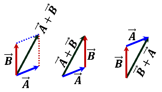 $\vec{A}\pm \vec{B}=\pm ~\vec{B}+\vec{A}$ $\vec{A}\pm \vec{B}=\pm ~\vec{B}+\vec{A}$ 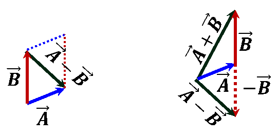 |
Cartesian |
$\vec{A}\pm \vec{B}={{A}_{x}}~\overrightarrow{{{a}_{x}}}+{{A}_{y}}~\overrightarrow{{{a}_{y}}}+{{A}_{z}}~\overrightarrow{{{a}_{z}}}\pm \left( {{B}_{x}}~\overrightarrow{{{a}_{x}}}+{{B}_{y}}~\overrightarrow{{{a}_{y}}}+{{B}_{z}}~\overrightarrow{{{a}_{z}}} \right)=\left( {{A}_{x}}\pm {{B}_{x}} \right)~\overrightarrow{{{a}_{x}}}+\left( {{A}_{y}}\pm {{B}_{y}} \right)~\overrightarrow{{{a}_{y}}}+\left( {{A}_{z}}\pm {{B}_{z}} \right)~\overrightarrow{{{a}_{z}}}$ |
Cylindrical |
$\vec{A}\pm \vec{B}=\left( {{A}_{\rho }}~\overrightarrow{{{a}_{\rho A}}}+{{A}_{z}}~\overrightarrow{{{a}_{z}}} \right)\pm \left( {{B}_{\rho }}~\overrightarrow{{{a}_{\rho B}}}+{{B}_{z}}~\overrightarrow{{{a}_{z}}} \right)$$=\left( {{A}_{\rho }}\overrightarrow{{{a}_{\rho A}}}\pm {{B}_{\rho }}\overrightarrow{{{a}_{\rho B}}} \right)+\left( {{A}_{z}}\pm {{B}_{z}} \right)\overrightarrow{{{a}_{z}}}$ $=\left( {{A}_{x}}\pm {{B}_{x}} \right)~\overrightarrow{{{a}_{x}}}+\left( {{A}_{y}}\pm {{B}_{y}} \right)~\overrightarrow{{{a}_{y}}}+\left( {{A}_{z}}\pm {{B}_{z}} \right)~\overrightarrow{{{a}_{z}}}$ |
Spherical |
$\vec{A}\pm \vec{B}~=\left( {{A}_{r}}\overrightarrow{{{a}_{rA}}}\pm {{B}_{r}}\overrightarrow{{{a}_{rB}}} \right)~=\left( {{A}_{x}}\pm {{B}_{x}} \right)~\overrightarrow{{{a}_{x}}}+\left( {{A}_{y}}\pm {{B}_{y}} \right)~\overrightarrow{{{a}_{y}}}+\left( {{A}_{z}}\pm {{B}_{z}} \right)~\overrightarrow{{{a}_{z}}}$ |
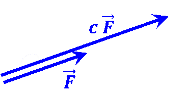
Table 3.6 – Vector Scaling
Scaling |
 |
Cartesian |
$c~\left( {{A}_{x}}~\overrightarrow{{{a}_{x}}}+{{A}_{y}}~\overrightarrow{{{a}_{y}}}+{{A}_{z}}~\overrightarrow{{{a}_{z}}} \right)=c{{A}_{x}}~\overrightarrow{{{a}_{x}}}+c{{A}_{y}}~\overrightarrow{{{a}_{y}}}+c{{A}_{z}}~\overrightarrow{{{a}_{z}}}$ |
Cylindrical |
$c~\left( {{A}_{\rho }}~\overrightarrow{{{a}_{\rho }}}+{{A}_{z}}~\overrightarrow{{{a}_{z}}} \right)=c{{A}_{\rho }}~\overrightarrow{{{a}_{\rho }}}+c{{A}_{z}}~\overrightarrow{{{a}_{z}}}$ |
Spherical |
$c~\left( {{A}_{r}}~\overrightarrow{{{a}_{r}}} \right)=c{{A}_{r}}~\overrightarrow{{{a}_{r}}}$ |
Table 3.7 – Vector Dot Product
Scalar (Dot) Product |
W = Work Done by force ${\vec{F} }~{ along }~{ the }~{ path }~{ }\vec{\ell }$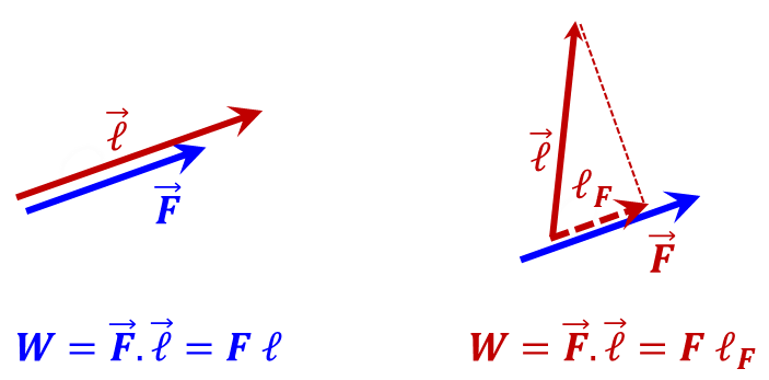 |
I = Current flow through the surface ${\vec{S} }~{ }~{ due }~{ to}~{area}~{density}~~\mathbf{\vec{J}}$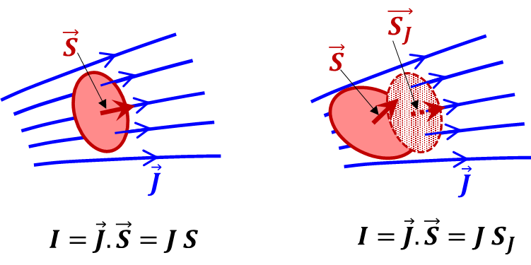 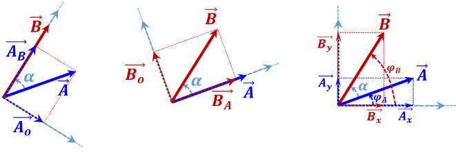 ${\vec{A}}\cdot {\vec{B}}=\left[ {{{A}}_{{B}}} \right]{ }~{ B}=\left[ {A }~{ cos}\left( { }\alpha{ } \right) \right]{ }~{ B}={A }~{ B }~{ cos}\left( { }\alpha{ } \right)$ ${\vec{A}}\cdot {\vec{B}}={A }~{ }\left[ {{{B}}_{{A}}} \right]{ }~{ }={A }~{ }\left[ {B }~{ cos}\left( { }\alpha{ } \right) \right]{ }~{ }={A }~{ B }~{ cos}\left( { }\alpha{ } \right)$ ${\vec{A}}\cdot {\vec{B}}={{{A}}_{{x}}}{{{B}}_{{x}}}+{{{A}}_{{y}}}{{{A}}_{{y}}}=\left[ {A }~{ cos}\left( {{{ }\varphi{ }}_{{A}}} \right){B }~{ cos}\left( {{{ }\varphi{ }}_{{B}}} \right)+{A }~{ sin}\left( {{{ }\varphi{ }}_{{A}}} \right){B }~{ sin}\left( {{{ }\varphi{ }}_{{B}}} \right) \right]={A }~{ B }~{ }\left[ {cos}\left( {{{ }\varphi{ }}_{{A}}} \right){cos}\left( {{{ }\varphi{ }}_{{B}}} \right)+{sin}\left( {{{ }\varphi{ }}_{{A}}} \right){sin}\left( {{{ }\varphi{ }}_{{B}}} \right) \right] \\ ={AB}\left[ {cos}\left( {{{ }\varphi{ }}_{{B}}}-{{{ }\varphi{ }}_{{A}}} \right) \right] \\ ={A }~{ B }~{ cos}\left( { }\alpha{ } \right)$ |
|
Cartesian |
${\vec{A}}\cdot {\vec{B}}=\left( {{{A}}_{{x}}}{ }~{ }\overrightarrow{{{{a}}_{{x}}}}+{{{A}}_{{y}}}{ }~{ }\overrightarrow{{{{a}}_{{y}}}}+{{{A}}_{{z}}}{ }~{ }\overrightarrow{{{{a}}_{{z}}}} \right)\cdot \left( {{{B}}_{{x}}}{ }~{ }\overrightarrow{{{{a}}_{{x}}}}+{{{B}}_{{y}}}{ }~{ }\overrightarrow{{{{a}}_{{y}}}}+{{{B}}_{{z}}}{ }~{ }\overrightarrow{{{{a}}_{{z}}}} \right)={{{A}}_{{x}}}{ }~{ }{{{B}}_{{x}}}+{{{A}}_{{y}}}{ }~{ }{{{B}}_{{y}}}+{{{A}}_{{z}}}{ }~{ }{{{B}}_{{z}}}$ |
Cylindrical |
${\vec{A}}\cdot {\vec{B}}=\left( {{{A}}_{{ }\rho{ }}}{ }~{ }\overrightarrow{{{{a}}_{{ }\rho{ A}}}}+{{{A}}_{{z}}}{ }~{ }\overrightarrow{{{{a}}_{{z}}}} \right)\cdot \left( {{{B}}_{{ }\rho{ }}}{ }~{ }\overrightarrow{{{{a}}_{{ }\rho{ B}}}}+{{{B}}_{{z}}}{ }~{ }\overrightarrow{{{{a}}_{{z}}}} \right)={{{A}}_{{ }\rho{ }}}{{{B}}_{{ }\rho{ }}}\left( \overrightarrow{{{\mathbf{a}}_{\mathbf{\rho A}}}}\cdot \overrightarrow{{{\mathbf{a}}_{\mathbf{\rho B}}}} \right)+{{{A}}_{{z}}}{ }~{ }{{{B}}_{{z}}}$ |
Spherical |
${\vec{A}}\cdot {\vec{B}}=\left( {{{A}}_{{r}}}{ }~{ }\overrightarrow{{{{a}}_{{rA}}}} \right)\cdot \left( {{{B}}_{{r}}}{ }~{ }\overrightarrow{{{{a}}_{{rB}}}} \right)={{{A}}_{{r}}}{{{B}}_{{r}}}\left( \overrightarrow{{{\mathbf{a}}_{\mathbf{rA}}}}\cdot \overrightarrow{{{\mathbf{a}}_{\mathbf{rB}}}} \right)$ |
Table 3.8 – Vector Cross Product
Vector (Cross) Product |
${\vec{T}}$ = Torque vector due to a force ${\vec{F} }~{ and }~{ an }~{ arm }~{ \vec{d}}$ 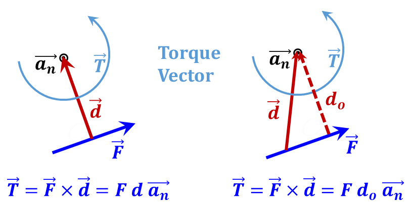 |
$\mathbf{\vec{S}}=$ Area vector of a parallelogram with sides ${\vec{w} }~{ and }~{ }\vec{\ell }$ 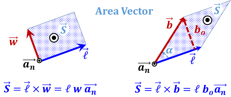 |
|
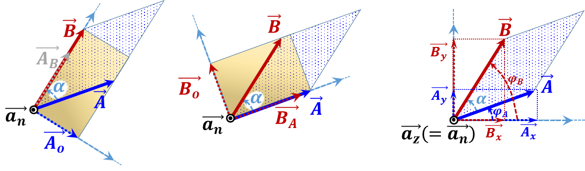 ${\vec{A}}\times {\vec{B}}=\left[ {{{A}}_{{o}}} \right]{ }~{ B }~{ }\overrightarrow{{{{a}}_{{n}}}}=\left[ {A }~{ sin}\left( { }\alpha{ } \right) \right]{ }~{ B }~{ }\overrightarrow{{{{a}}_{{n}}}}={A }~{ B }~{ sin}\left( { }\alpha{ } \right)$ $\overrightarrow{{{{a}}_{{n}}}}$ ${\vec{A}}\times {\vec{B}}={A }~{ }\left[ {{{B}}_{{o}}} \right]{ }~{ }\overrightarrow{{{{a}}_{{n}}}}={A }~{ }\left[ {B }~{ sin}\left( { }\alpha{ } \right) \right]{ }~{ }\overrightarrow{{{{a}}_{{n}}}}={A }~{ B }~{ sin}\left( { }\alpha{ } \right)$ $\overrightarrow{{{{a}}_{{n}}}}$ ${\vec{A}}\times {\vec{B}}=\left[ {{{A}}_{{x}}}{{{B}}_{{y }~{ }}}\overrightarrow{{{{a}}_{{n}}}}+{{{A}}_{{y}}}{{{B}}_{{x}}}\left( -\overrightarrow{{{{a}}_{{n}}}} \right) \right]=\left[ {A }~{ cos}\left( {{{ }\varphi{ }}_{{A}}} \right){Bsin}\left( {{{ }\varphi{ }}_{{B}}} \right)-{A }~{ sin}\left( {{{ }\varphi{ }}_{{A}}} \right){B }~{ cos}\left( {{{ }\varphi{ }}_{{B}}} \right) \right]{ }~{ }\overrightarrow{{{{a}}_{{n}}}}={A }~{ B }~{ }\left[ {cos}\left( {{{ }\varphi{ }}_{{A}}} \right){sin}\left( {{{ }\varphi{ }}_{{B}}} \right)-{sin}\left( {{{ }\varphi{ }}_{{A}}} \right){cos}\left( {{{ }\varphi{ }}_{{B}}} \right) \right]{ }~{ }\overrightarrow{{{{a}}_{{n}}}} \\ ~~~~~~~~~ ={AB}\left[ {sin}\left( {{{ }\varphi{ }}_{{B}}}-{{{ }\varphi{ }}_{{A}}} \right) \right]{ }~{ }\overrightarrow{{{{a}}_{{n}}}} \\ ~~~~~~~~~ ={A }~{ B }~{ sin}\left( { }\alpha{ } \right){ }~{ }\overrightarrow{{{{a}}_{{n}}}}$ |
|
| ${\vec{A}}\times {\vec{A}}=0$ , ${\vec{A}}\times {\vec{B}}=-{\vec{B}}\times {\vec{A}}$ | |
Cartesian |
$\overrightarrow{{{{a}}_{{x}}}}\times \overrightarrow{{{{a}}_{{y}}}}=\overrightarrow{{{{a}}_{{z}}}}$ , $\overrightarrow{{{{a}}_{{y}}}}\times \overrightarrow{{{{a}}_{{z}}}}=\overrightarrow{{{{a}}_{{x}}}}$ , $\overrightarrow{{{{a}}_{{z}}}}\times \overrightarrow{{{{a}}_{{x}}}}=\overrightarrow{{{{a}}_{{y}}}}$ ${\vec{A}}\times {\vec{B}}=\left( {{{A}}_{{x}}}{ }~{ }\overrightarrow{{{{a}}_{{x}}}}+{{{A}}_{{y}}}{ }~{ }\overrightarrow{{{{a}}_{{y}}}}+{{{A}}_{{z}}}{ }~{ }\overrightarrow{{{{a}}_{{z}}}} \right)\times \left( {{{B}}_{{x}}}{ }~{ }\overrightarrow{{{{a}}_{{x}}}}+{{{B}}_{{y}}}{ }~{ }\overrightarrow{{{{a}}_{{y}}}}+{{{B}}_{{z}}}{ }~{ }\overrightarrow{{{{a}}_{{z}}}} \right)=\left| \begin{matrix} \overrightarrow{{{{a}}_{{x}}}} & \overrightarrow{{{{a}}_{{y}}}} & \overrightarrow{{{{a}}_{{z}}}} \\ {{{A}}_{{x}}} & {{{A}}_{{y}}} & {{{A}}_{{z}}} \\ {{{B}}_{{x}}} & {{{B}}_{{y}}} & {{{B}}_{{z}}} \\ \end{matrix} \right|$ |
Cylindrical |
$\overrightarrow{{{{a}}_{{ }\rho{ }}}}\times \overrightarrow{{{{a}}_{{ }\varphi{ }}}}=\overrightarrow{{{{a}}_{{z}}}}$ , $\overrightarrow{{{{a}}_{{ }\varphi{ }}}}\times \overrightarrow{{{{a}}_{{z}}}}=\overrightarrow{{{{a}}_{{ }\rho{ }}}}$ , $\overrightarrow{{{{a}}_{{z}}}}\times \overrightarrow{{{{a}}_{{ }\rho{ }}}}=\overrightarrow{{{{a}}_{{ }\varphi{ }}}}$ ${\vec{A}}\times {\vec{B}}=\left( {{{A}}_{{ }\rho{ }}}{ }~{ }\overrightarrow{{{{a}}_{{ }\rho{ A}}}}+{{{A}}_{{z}}}{ }~{ }\overrightarrow{{{{a}}_{{z}}}} \right)\times \left( {{{B}}_{{ }\rho{ }}}{ }~{ }\overrightarrow{{{{a}}_{{ }\rho{ B}}}}+{{{B}}_{{z}}}{ }~{ }\overrightarrow{{{{a}}_{{z}}}} \right) \\ ~~~~~~~~~ ={{{A}}_{{ }\rho{ }}}{{{B}}_{{ }\rho{ }}}\left( \overrightarrow{{{\mathbf{a}}_{\mathbf{\rho A}}}}\times \overrightarrow{{{\mathbf{a}}_{\mathbf{\rho B}}}} \right)+\left( {{{A}}_{{ }\rho{ }}}{{{B}}_{{z}}}{ }~{ }\overrightarrow{{{{a}}_{{ }\rho{ A}}}}\times \overrightarrow{{{{a}}_{{z}}}}+{{{A}}_{{z}}}{{{B}}_{{ }\rho{ }}}{ }~{ }\overrightarrow{{{{a}}_{{z}}}}\times \overrightarrow{{{{a}}_{{ }\rho{ B}}}} \right) \\ ~~~~~~~~~ ={{{A}}_{{ }\rho{ }}}{{{B}}_{{ }\rho{ }}}\left( \overrightarrow{{{\mathbf{a}}_{\mathbf{\rho A}}}}\times \overrightarrow{{{\mathbf{a}}_{\mathbf{\rho B}}}} \right)+\left( -{{{A}}_{{ }\rho{ }}}{{{B}}_{{z}}}{ }~{ }\overrightarrow{{{{a}}_{{ }\varphi{ A}}}}+{{{A}}_{{z}}}{{{B}}_{{ }\rho{ }}}{ }~{ }\overrightarrow{{{{a}}_{{ }\varphi{ B}}}} \right)$ |
Spherical |
$\overrightarrow{{{{a}}_{{r}}}}\times \overrightarrow{{{{a}}_{{ }\theta{ }}}}=\overrightarrow{{{{a}}_{{ }\varphi{ }}}}$ , $\overrightarrow{{{{a}}_{{ }\theta{ }}}}\times \overrightarrow{{{{a}}_{{ }\varphi{ }}}}=\overrightarrow{{{{a}}_{{r}}}}$ , $\overrightarrow{{{{a}}_{{ }\varphi{ }}}}\times \overrightarrow{{{{a}}_{{r}}}}=\overrightarrow{{{{a}}_{{ }\theta{ }}}}$ ${\vec{A}}\times {\vec{B}}=\left( {{{A}}_{{r}}}{ }~{ }\overrightarrow{{{{a}}_{{rA}}}} \right)\times \left( {{{B}}_{{r}}}{ }~{ }\overrightarrow{{{{a}}_{{rB}}}} \right)={{{A}}_{{r}}}{{{B}}_{{r}}}\left( \overrightarrow{{{\mathbf{a}}_{\mathbf{rA}}}}\times \overrightarrow{{{\mathbf{a}}_{\mathbf{rB}}}} \right)$ |
Addendum III: Spatial Distributions and Densities
In the following we will discuss spatial distributions and densities of both static and dynamic quantities.
Static Distributions and Densities.
Static quantities, such as mass, charge, or energy, may exist in several possible spatial distributions, Figure 3.27:
1. A concentration in an infinitesimally small volume, which we typically represent as a "point".
2. A distribution over a volume with infinitesimally small cross-section, which we typically represent as a "line".
3. A distribution over a volume with infinitesimally small thickness, which we typically represent as a "surface".
4. A distribution over a volume with non-zero dimensions.
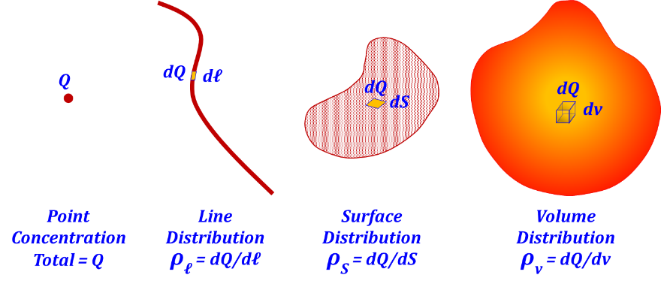
Figure 3.27
Figure 3.27
These distributions may or may not be uniform. To express their spatial features, we use appropriate density expressions such as volume, area, or linear density of the quantity distribution. Densities of static quantities are scalar in nature, i.e. have only magnitudes and do not have directions. We will use the subscripted $ρ_{v}, ρ_{S}$, and $ρ_{ℓ}$ to denote volume, area, and linear densities, respectively. Hence, for the static quantity Q, we can write
${{{ }\rho{ }}_{{v}}}=\frac{{dQ}}{{dv}}{ }~{ },{ }~{ }{{{ }\rho{ }}_{{S}}}=\frac{{dQ}}{{dS}}{ }~{ },{ }~{ and }~{ }{{{ }\rho{ }}_{\ell }}=\frac{{dQ}}{{d}\ell }{ }~{ } \tag {3.9}$
For uniform distributions, the density is constant at all the distribution locations, otherwise, the density would be a function of position. Depending on the case, these densities may or may not have physical relevance and their definition could be meaningless. Examples are defining a volumetric density for a point concentration where the volume is zero, or defining the linear density for a spherical volume distribution. The following table summarizes the corresponding densities for the four distribution forms.
Table 3.9 – Static Distribution Densities
|
Configuration |
Volume Density= Quantity per unit volume |
Surface Density= Quantity per unit area |
Linear Density= Quantity per unit length |
|
Point Concentration |
Zero volume → $ρ_{v}$ = ∞ |
Zero area → $ρ_{S}$ = ∞ |
Zero length → $ρ_{ℓ}$ = ∞ |
|
Line Distribution |
Zero volume → $ρ_{v}$ = ∞ |
Zero area → $ρ_{S}$ = ∞ |
$ρ_{ℓ}$ |
|
Surface Distribution |
Zero volume → $ρ_{v}$ = ∞ |
$ρ_{S}$ |
(Atypical?) |
|
Volume Distribution |
$ρ_{v}$ |
(Atypical?) |
(Atypical?) |
Conversions between static density expressions:
In some distribution configurations, more than one form of density can be simultaneously defined. An example is a cylindrical volume distribution for which a volumetric density can be defined while a linear density along the cylindrical axis can be defined as well. For such cases, it is useful to have conversion expressions between the different forms. In the following, we provide examples of such conversion relationships.
Table 3.10
Non uniform distribution |
Uniform distribution |
|
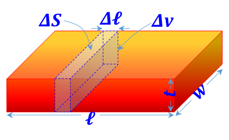
| Sheet distribution ${{{ }\rho{ }}_{{S}}}=\frac{{dQ}}{{dS}}$ is defined |
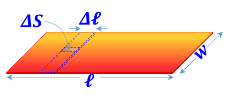 $ {{{ }\rho{ }}_{\ell }}=\frac{\mathop{\int }_{{w}}{{{ }\rho{ }}_{{S}}}{ }~{ dS}}{\Delta \ell }=\underset{{w}}{\mathop \int }\,{{{ }\rho{ }}_{{S}}}{ }~{ dw}$ |
 ${{{ }\rho{ }}_{\ell }}={{{ }\rho{ }}_{{S}}}{ }~{ w}$ |
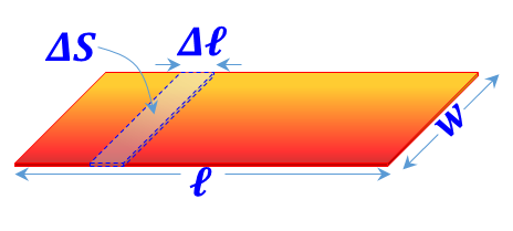
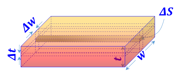
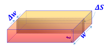
| Rectangular prism
(Slab) distribution ${{{ }\rho{ }}_{{v}}}=\frac{{dQ}}{{dv}}$ is defined |
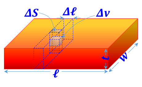 ${{{ }\rho{ }}_{{S}}}=\frac{\mathop{\int }_{{t}}{{{ }\rho{ }}_{{v}}}{ }~{ dv}}{\Delta {S}}=\underset{{t}}{\mathop \int }\,{{{ }\rho{ }}_{{S}}}{ }~{ dt}$ ${{{ }\rho{ }}_{\ell }}=\frac{\mathop{\int }_{{w}}\mathop{\int }_{{t}}{{{ }\rho{ }}_{{v}}}{ }~{ dv}}{\Delta \ell }=\underset{{w}}{\mathop \int }\,\underset{{t}}{\mathop \int }\,{{{ }\rho{ }}_{{v}}}{ }~{ dt }~{ dw}$ |
 ${{{ }\rho{ }}_{{S}}}={{{ }\rho{ }}_{{S}}}{ }~{ t}$ ${{{ }\rho{ }}_{\ell }}={{{ }\rho{ }}_{{v}}}{ }~{ t }~{ w}$ |
| Circular prism
(Cylinder) distribution ${{{ }\rho{ }}_{{v}}}=\frac{{dQ}}{{dv}}$ is defined |
 ${{{ }\rho{ }}_{\ell }}=\frac{\mathop{\int }_{{S}}{{{ }\rho{ }}_{{v}}}{ }~{ dv}}{\Delta \ell }=\underset{{S}}{\mathop \int }\,{{{ }\rho{ }}_{{v}}}{ }~{ dS}$ |
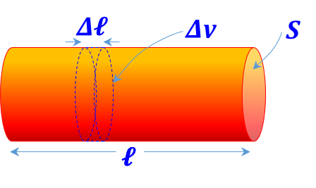 ${{{ }\rho{ }}_{\ell }}={{{ }\rho{ }}_{{v}}}{ }~{ S}$ |
Dynamic Distributions and Densities:
Examples of dynamic quantities include electric current, air current, fluid flow, and energy flow. Spatial distributions for a dynamic flow can only exist in one of the following forms, Figure 3.28:
1. A stream distribution with infinitesimally small cross-section, which we typically represent as a "line current/flow".
2. A stream distribution with infinitesimally small thickness, which we typically represent as a "surface current / laminar flow".
3. A stream distribution with non-zero cross-sectional area, "volume current/flow".
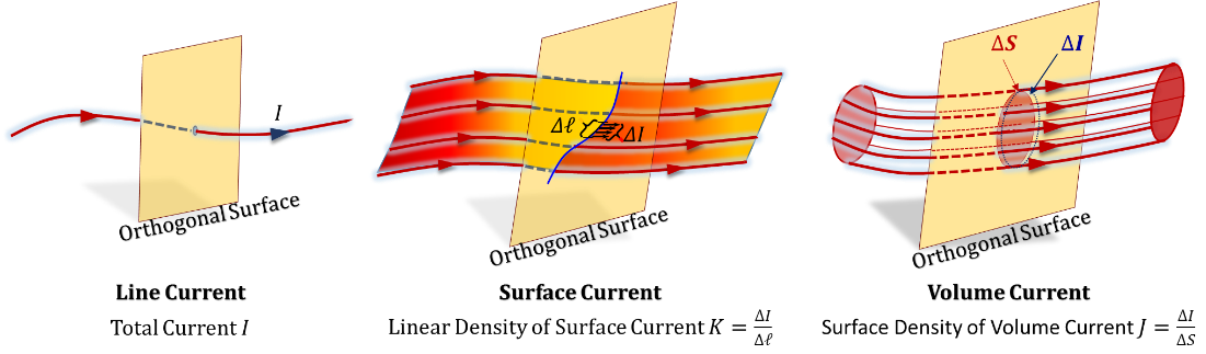
Figure 3.28
Figure 3.28
These distributions may or may not be uniform. To express their spatial features, in both magnitude and direction, we use appropriate vector density expressions.
${\vec{J}}=\frac{{dI}}{{d}{{{S}}_{{n}}}}{{{\vec{a}}}_{{I}}}{ }~{ }~{ }~{ }~{ }~{ and }~{ }~{ }~{ }~{ }~{ \vec{K}}=\frac{{dI}}{{d}{{\ell }_{{n}}}}{ }~{ }{{{\vec{a}}}_{{I}}} \tag {3.10}$
where the n subscripts indicate that both $dℓ$ and $dS$ must be orthogonal to the flow and ${{\vec{a}}_{I}}$ is the unit vector along the current/flow direction. For uniform distributions, the densities are constant at all the distribution locations, otherwise, the density would be a function of position. Again, depending on the case, these densities may or may not have physical relevance and their definition could be meaningless. The following table summarizes the corresponding densities for dynamic distributions.
Table 3.11 – Dynamic Distribution Densities
|
Configuration |
Area Density= Quantity per unit area |
Linear Density= Quantity per unit length |
|
Line Stream Concentration |
Zero area → ${\vec{J}}$ = ∞ |
Zero length → ${\vec{K}}$= ∞ |
|
Surface Stream Distribution |
Zero area → ${\vec{J}}$= ∞ |
${\vec{K}}$ |
|
Volume Stream Distribution |
${\vec{J}}$ |
(Atypical?) |
Conversions between dynamic density expressions:
In this section, we demonstrate the relationship between the two forms of dynamic distribution densities in cases where both can be simultaneously defined. In the table below, we the example of a stream distribution in a slab configuration and the corresponding conversion relationships.
Table 3.12
Non uniform distribution |
Uniform distribution n |
|
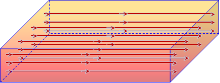 Slab Stream Flow/Current ${\vec{J}}=\frac{{dI}}{{d}{{{S}}_{{n}}}}{{{\vec{a}}}_{{I}}}$ is defined |
 ${\vec{K}}=\frac{\mathop{\int }_{{t}}{J }~{ dS}}{\Delta {w}}{ }~{ }{{{\vec{a}}}_{{I}}}=\underset{{t}}{\mathop \int }\,{J }~{ dt }~{ }{{{\vec{a}}}_{{I}}}$ |
 ${\vec{K}}={J }~{ t }~{ }{{{\vec{a}}}_{{I}}}$ |
Addendum IV: Line, Surface, and Volume Integrations
Introduction
In the course of this book, as we deal with various physical phenomena, analyses involving integration of scalar and vector quantities is common. We often need to carry out contour (or line) integrations, integrations over an area of a surface, a closed surface as well as volume integrations. Our background in mathematics should enable us to carry most of these integrations once they are set up properly. We can also resort to integration tables, computer software packages, or even numerical tools for "difficult" integrations. Hence, in this addendum, we will focus on two aspects of the issue that are often the obstacle. One is how to set up the integration equation starting with the physical problem, and the second is how to deal with vector quantities within the integrand.
The first obstacle of setting up the integral is an "integral" part of setting up the proper mathematical model of the physical problem. This is an acquired skill that the learners in this field acquire with practice. The learner needs to get exposed to a variety of cases and a variety of analysis tools to appreciate what works and what does not and when to use a specific model and what are the constraints of that use. Gaining this skill requires proper appreciation to the physics of the subject and good command of relevant mathematical tools. This will be demonstrated and emphasized throughout the different chapters of this book.
We now turn to dealing with integrations containing vector quantities. This will be followed by an overview/survey of line, surface, and volume "scalar" integrations.
Integrating vector quantities
To integrate vector quantities is simply performing vector summation of incremental vector elements. Since the sum of vectors is controlled by the directions of the vectors involved, the process of vector integration must take into account the variability of the direction of the vectors being integrated. Let us start with a "sarcastic" but true statement by saying that "The proper way of handling vector integration is not to do vector integration." What is meant here is that we should not start the integration process before we remove all vector quantities from within the integrand.
The process involves finding ways to get all vector terms outside the integration sign leaving only scalar quantities inside the integration. To extract a term outside the integral operator, this term must be a constant. Hence, what we must do is express all variable-direction vectors in terms of fixed-direction vectors that can then be extracted outside the integration. Let us cite some examples to demonstrate.
Example of a Cartesian coordinate Integral
$\int \vec{x}~dx=\int x~{{\vec{a}}_{x}}~dx={{\vec{a}}_{x}}\int x~~dx={{\vec{a}}_{x}}\left( \frac{{{x}^{2}}}{2}+c \right) \tag {3.11}$
$\int \vec{y}~dx=\int y~{{\vec{a}}_{y}}~dx={{\vec{a}}_{y}}\int y~~dx \tag {3.12}$
Example of a Cylindrical coordinate Integral
$\int \vec{\rho }~d\rho =\int \rho ~{{\vec{a}}_{\rho }}~d\rho ={{\vec{a}}_{\rho }}\int \rho ~~d\rho ={{\vec{a}}_{\rho }}\left( \frac{{{\rho }^{2}}}{2}+c \right) \tag {3.13}$
For an integration along $dρ$, the "${{\vec{a}}_{\rho }}$" has a constant direction and hence it is a constant vector that can be taken outside the integration. However if the same integration was along $d$φ, the "${{\vec{a}}_{\rho }}$" will vary as we vary φ and hence "${{\vec{a}}_{\rho }}$" needs to be expressed in terms of other constant-direction vectors to be able to carry out the integration. Logically, we use the Cartesian unit vectors "${{\vec{a}}_{x}},~{{\vec{a}}_{y}},~and~{{\vec{a}}_{z}}$'' which are always constant vectors in this regard,
$\int \vec{\rho }~d\varphi =\int \rho ~{{\vec{a}}_{\rho }}~d\varphi =\int \rho ~\left( \cos \varphi ~\overrightarrow{{{a}_{x}}}+\sin \varphi ~\overrightarrow{{{a}_{y}}} \right)~d\varphi =\int \rho ~\left( \cos \varphi ~\overrightarrow{{{a}_{x}}} \right)~d\varphi + \\ \int \rho ~\left( \sin \varphi ~\overrightarrow{{{a}_{y}}} \right)~d\varphi =\overrightarrow{{{a}_{x}}}\int \rho ~\left( \cos \varphi \right)~d\varphi +\overrightarrow{{{a}_{y}}}\int \rho \left( \sin \varphi \right)~d\varphi =\overrightarrow{{{a}_{x}}}~\left( \rho \sin \varphi +{{c}_{1}} \right)- \\ \overrightarrow{{{a}_{y}}}~\rho ~\left( \cos \varphi +{{c}_{2}} \right)\tag {3.14}$
Adding the limits between 0 and 2π, this integration reduces to:
$\underset{0}{\overset{2\pi }{\mathop \int }}\,\vec{\rho }~d\varphi =\overrightarrow{{{a}_{x}}}~~\rho \underset{0}{\overset{2\pi }{\mathop \int }}\,\left( \cos \varphi \right)~d\varphi +\overrightarrow{{{a}_{y}}}~\rho \underset{0}{\overset{2\pi }{\mathop \int }}\,\left( \sin \varphi \right)~d\varphi =0 \tag {3.15}$
This result makes physical sense since adding the variable direction vector $\vec{\rho }$ around a complete 2π (360 degrees) rotation will produce zero net,
see Figure 3.29.
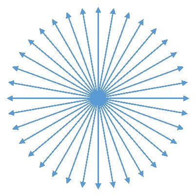
Figure 3.29
Figure 3.29
Example of a Spherical coordinate Integral
$\int \vec{r}~dr=\int r~{{\vec{a}}_{r}}~dr={{\vec{a}}_{r}}\int r~dr={{\vec{a}}_{r}}~\left( {{r}^{2}}/2 \right)\tag {3.16}$
$\int \vec{r}~d\theta =\int r~{{\vec{a}}_{r}}~d\theta =\int r~\left( \sin \theta \cos \varphi ~\overrightarrow{{{a}_{x}}}+\sin \theta \sin \varphi ~\overrightarrow{{{a}_{y}}}+\cos \theta \overrightarrow{{{a}_{z}}} \right)~d\theta = \\ \overrightarrow{{{a}_{x}}}\int r\sin \theta \cos \varphi d\theta +\overrightarrow{{{a}_{y}}}\int r\sin \theta \sin \varphi d\theta +\overrightarrow{{{a}_{z}}}\int r\cos \theta d\theta \tag {3.17}$
Integrating scalar quantities
In this section, we will survey a few examples of line, surface and volume integrations that we will find relevant in the chapters ahead.
Examples of Density Integrations:
Two types of densities are reviewed here; static and dynamic. Examples of static densities include mass and charge distributions, while examples of dynamic densities include fluid flow and electric current.
Static Linear Density
If ${{\rho }_{\ell }}\left( position \right)$ is the linear density of the distribution of a quantity Q, we can obtain the total Q by integrating the linear density over the length of the distribution.
$Q=\int dQ=\int \frac{dQ}{d\ell }~d\ell =\int {{\rho }_{\ell }}~d\ell \tag {3.18}$
Static Surface Density
If ${{\rho }_{\text{S}}}\left( position \right)$ is the surface density of the distribution of a quantity Q, we can obtain the total Q by integrating the surface density over the area of the distribution.
$Q=\int dQ=\iint \frac{dQ}{dS}~dS=\iint {{\rho }_{S}}~dS \tag {3.19}$
Static Volumetric Density
If is the volumetric density of the distribution of a quantity Q, we can obtain the total Q by integrating the volumetric density over the volume of the distribution.
$Q=\int dQ=\int\!\!\int\!\!\int \frac{dQ}{dv}~dv=\int\!\!\int\!\!\int {{\rho }_{v}}~dv \tag {3.20}$
Dynamic Linear Density
If ${{K}_{\ell }}\left( position \right)$ is the linear density of the distribution of a current (flow) I, we can obtain the total I by integrating the linear density across the cross-sectional length of the distribution. The cross-sectional length is a length orthogonal to the flow distribution, Figure 3.30.
$I=\int dI=\int \frac{dI}{d\ell }~d\ell =\int {{K}_{\ell }}~d\ell \tag {3.21}$
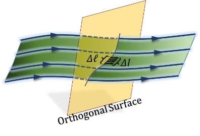
Figure 3.30
Figure 3.30
Dynamic Surface Density
The total flow (current), I, flowing through a specific surface is the integration of the flow surface density ($J = dI/dS$) over the cross-sectional surface area of interest. The cross-sectional area is that of a surface orthogonal to the flow distribution, Figure 3.31.
$I=\int dI=\iint \frac{dI}{dS}~dS=\iint J~dS \tag {3.22}$
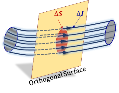
Figure 3.31
Figure 3.31
Examples of Work and Energy Integrations:
The work done by a force acting on an object as it moves an unconstrained object a certain distance (along the action line of the force), see Figure 3.32.
$W=\int dW=\int F~d\ell \tag {3.23}$
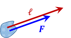
Figure 3.32
Figure 3.32
The total energy stored in a specific volume is the integration of the volumetric energy density ($w = dU/dv$) over the volume of interest.
$U=\int dU=\int \!\!\int \!\!\int \frac{dU}{dv}~dv=\int \!\!\int \!\!\int w~dv \tag {3.24}$
Table 3.13 – Examples of integrations in different coordinate systems
|
Line: $\int F~d\ell $ |
Surface: $\int \!\!\int J~dS$ |
Volume: $\int \!\!\int \!\!\int w~dv$ |
|
|
Cartesian |
$\int F\left( x,y,z \right)~dx$ |
$\int \!\!\int J\left( x,y,z \right)~dydz$ |
$\int\!\! \int \!\!\int w\left( x,y,z \right)~dx~dy~dz$ |
|
$\int F\left( x,y,z \right)~dy$ |
$\int \!\!\int J\left( x,y,z \right)~dzdx$ |
||
|
$\int F\left( x,y,z \right)~dz$ |
$\int\!\! \int J\left( x,y,z \right)~dxdy$ |
||
|
Cylindrical |
$\int F\left( \rho ,\varphi ,z \right)~d\rho $ |
$\int\!\! \int J\left( \rho ,\varphi ,z \right)~\rho d\varphi ~dz$ |
$\int \!\!\int \!\!\int w\left( \rho ,\varphi ,z \right)~d\rho ~\rho d\varphi ~dz$ |
|
$\int F\left( \rho ,\varphi ,z \right)~\rho ~d\varphi $ |
$\int\!\! \int J\left( \rho ,\varphi ,z \right)~dz~d\rho $ |
||
|
$\int F\left( \rho ,\varphi ,z \right)~dz$ |
$\int \!\!\int J\left( \rho ,\varphi ,z \right)~d\rho ~\rho d\varphi $ |
||
|
Spherical |
$\int F\left( r,\theta ,\varphi \right)~dr$ |
$\int\!\! \int J\left( r,\theta ,\varphi \right)~rd\theta ~rsin\theta ~d\varphi $ |
$\int\!\! \int \!\!\int w\left( r,\theta ,\varphi \right)~dr~rd\theta ~rsin\theta ~d\varphi $ |
|
$\int F\left( r,\theta ,\varphi \right)~r~d\theta $ |
$\int \!\!\int J\left( r,\theta ,\varphi \right)~dr~rsin\theta ~d\varphi $ |
||
|
$\int F\left( r,\theta ,\varphi \right)~r~sin\theta ~d\varphi $ |
$\int \!\!\int J\left( r,\theta ,\varphi \right)~dr~rd\theta $ |
- Which vector operation measures the degree of colinearity (parallelism) between two vectors?
- Which vector operation measure the degree of perpendicularity between two vectors?
- Which fundamental physical phenomenon corresponds to a capacitor circuit component?
- Which fundamental physical phenomenon corresponds to an inductor circuit component?
Return to Lesson
Return to Video
Examples III.2
- Convert the vector field $x/\sqrt{(x^2+y^2)}{\vec{a}}_{x}+y/\sqrt{(x^2+y^2)}{\vec{a}}_{y}$ to cylindrical coordinates? Plot this vector field on the unit circle in the 2-D plane.
- Find the sum of a vector $(2,1,1)$ given in cylindrical coordinates and a vector $(2,3,1)$ given in rectangular coordinates at a point location $(1,2,1)$ in rectangular coordinates.
- Given the vector field $\vec{E}=\left\{ 4\,z\,{{y}^{2}}\,cos(2x) \right\}\,{{\vec{a}}_{x}}+\left\{ 2\,z\,y\,sin(x) \right\}\,{{\vec{a}}_{y}}+\left\{ {{y}^{2}}\,sin(x) \right\}\,{{\vec{a}}_{z}}$, for the region $|x|<1$, $|y|<1$ and $|z|<1$, find
- the surface on which the ${\vec{a}}_{y}$ component of the field equals $0$,
- the region on which the ${\vec{a}}_{y}$ component and the ${\vec{a}}_{z}$ component are equal.
Return to Lesson
Return to Video
Problems III.2
- A field is given as $\vec{G}=[25/({{x}^{2}}+{{y}^{2}})][x\ {{\vec{a}}_{x}}+y\ {{\vec{a}}_{y}}]$. Find
- a unit vector in the direction of ${\vec{G}}$ at a point $(3,~4,~-2)$
- the angle between ${\vec{G}}$ and ${{\vec{a}}_{x}}$ at the given point location.
- Find
- the vector component of $\vec{E}=10\,{{\vec{a}}_{x}}-6\,{{\vec{a}}_{y}}+5\,{{\vec{a}}_{z}}$ that is parallel to $\vec{G}=0.1\,{{\vec{a}}_{x}}-0.2\,{{\vec{a}}_{y}}+0.3\,{{\vec{a}}_{z}}$
- the vector component of ${\vec{F}}$ that is perpendicular to ${\vec{G}}$
- the vector component of ${\vec{G}}$ that is perpendicular to ${\vec{F}}$
- Find the normal to a surface containing the two vectors ${{\vec{x}}_{1}}=4\,{{\vec{a}}_{x}}-3\,{{\vec{a}}_{y}}+5\,{{\vec{a}}_{z}}$ and ${{\vec{x}}_{2}}=2\,{{\vec{a}}_{x}}-3\,{{\vec{a}}_{y}}+7\,{{\vec{a}}_{z}}$.