1. Read the lecture (displayed below) [30-60 minutes]
2. Watch the video    [24:28 minutes]
3. Do the exercises  [~30 minutes]

Total time = [~2:00 hours]

Last Lecture:

In lecture II.1, we carried out the Transmission Line Circuit Analysis Using the Distributed RLCG Model.

The line was assumed to extend along the $z$-axis, Figure 2.6. The input side (or the sending/transmitter end) to the TL was connected to a signal source with an internal "impedance" and at the receiving end at $z=\ell $ the line was connected to a load.

 

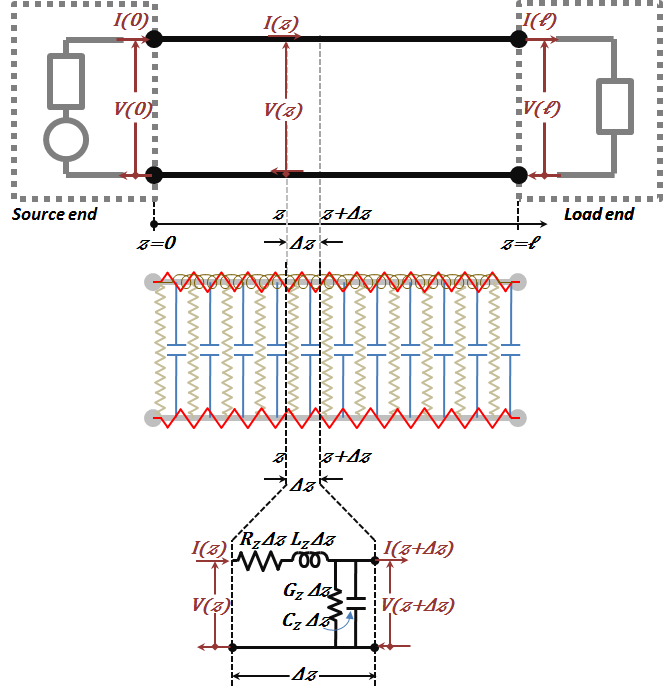
Figure 2.6

Using the distributed RLCG physically based model along with Kirchhoff's Voltage and Kirchhoff's Current Laws (KVL and KCL), we were able to write differential equations describing the voltage and current behaviors as functions of position $(z)$. This was performed in both time and frequency domains.

The steady-state harmonic analysis in the frequency domain yielded the following expressions for voltage and current expressions:

The corresponding time domain expressions are:

Also, we concluded that the expressions for case of lossless TL $({{R}_{z}}=0\text{ }\!\!~\!\!\text{ }and\text{ }\!\!~\!\!\text{ }{{G}_{z}}=0)$

Physical Implications of Solutions - $\alpha ,~\beta ,~\lambda ,~and~{{c}_{ph}}$:

At this point, it is important to take a pause to examine the obtained results and make sure that we relate to their physical implications.

We examine the harmonic solution obtained in the time domain:

$v\left( z,t \right)=\left| {{V}^{+}} \right|{{e}^{-\alpha z}}\cos \left( \omega t-\beta z+\varphi _{v}^{+} \right)+\left| {{V}^{-}} \right|{{e}^{+\alpha z}}\cos \left( \omega t+\beta z+\varphi _{v}^{-} \right)$

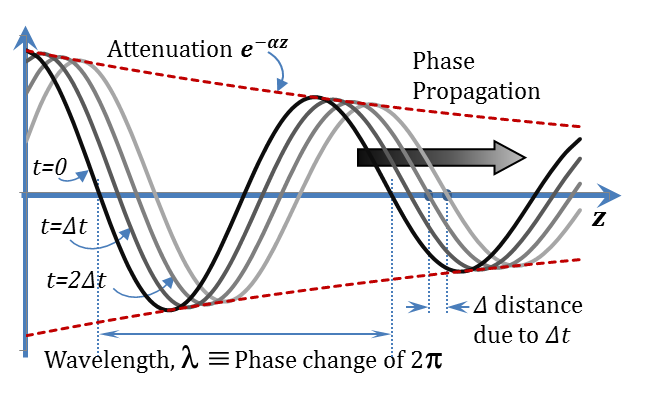
This solution has two terms. Let us take them one at a time: $\left| {{V}^{+}} \right|{{e}^{-\alpha z}}\cos \left( \omega t-\beta z+\varphi _{v}^{+} \right)$ describes a voltage wave that changes with both $t$ and $z$, a graph of which is shown in Figure 2.7

Figure 2.7

It is evident from the figure that this term represent a travelling wave that moves in the positive $z$ direction (and hence the plus superscript in denoting ${{V}^{+}}$). The wave amplitude attenuates (decays) exponentially with distance with an attenuation coefficient of ${{e}^{-\alpha z}}$.

The wave experiences a full cycle in a distance λ, and hence the corresponding phase change $\beta$λ should equal to $2\pi $. i. e. $\beta$λ =$2\pi $, or λ =$2\pi /\beta $.

The velocity of its phase propagation can be derived by monitoring the motion of a specific phase on the wave, $\omega {{t}_{1}}-\beta {{z}_{1}}+\varphi _{v}^{+}=\omega {{t}_{2}}-\beta {{z}_{2}}+\varphi _{v}^{+}~and~hence~\omega \,\Delta t=\beta \,\Delta z~,~or~\Delta z/\Delta t={{c}_{ph}}=\omega /\beta $

$Phase~velocity~{{c}_{ph}}=\frac{\omega }{\beta }=\frac{2\pi f}{\frac{2\pi }{\lambda }}=\lambda f \tag{2.36}$

With this definition for the phase velocity, the terms of Equations (2.29) can be rewritten as: $v\left( z,t \right)=\left| {{V}^{+}} \right|~{{e}^{-\alpha z}}~cos\left[ \omega \left( t-\frac{z}{{{c}_{ph}}} \right)+\varphi _{v}^{+} \right]+\left| {{V}^{-}} \right|~{{e}^{+\alpha z}}~cos\left[ \omega \left( t+\frac{z}{{{c}_{ph}}} \right)+\varphi _{v}^{-} \right]\tag{2.37}$

which makes Equation (2.34) for the lossless line reduce to:

$v\left( z,t \right)=\left| {{V}^{+}} \right|~cos\left[ \omega \left( t-\frac{z}{{{c}_{ph}}} \right)+\varphi _{v}^{+} \right]+\left| {{V}^{-}} \right|~~cos\left[ \omega \left( t+\frac{z}{{{c}_{ph}}} \right)+\varphi _{v}^{-} \right]\tag{2.38}$

Now, comparing this form to that obtained in the time domain for the lossless line in Equation (2.34), we conclude that the time argument $\left( t-\sqrt{{{L}_{z}}{{C}_{z}}}z \right)$ must be equivalent to $\left( t-\frac{z}{{{c}_{ph}}} \right)$ obtained in Equation (2.38), which implies that ${{c}_{ph}}=\frac{1}{\sqrt{{{L}_{z}}{{C}_{z}}}}\tag{2.39}$

Consequently, the time domain solution in the lossless line case, Equation (2.34), becomes: $v\left( z,t \right)={{v}^{+}}\left( t-\frac{z}{{{c}_{ph}}} \right)+{{v}^{-}}\left( t+\frac{z}{{{c}_{ph}}} \right)\tag{2.40}$

Now, back to the second term of the $v\left( z,t \right)$ solution $\left\{ \left| {{V}^{-}} \right|{{e}^{+\alpha z}}\cos \left( \omega t+\beta z+\varphi _{v}^{-} \right)=\left| {{V}^{-}} \right|\text{ }\!\!~\!\!\text{ cos}\left[ \omega \left( t+\frac{z}{{{c}_{ph}}} \right)+\varphi _{v}^{-} \right] \right\}$, Figure 2.8. This term represent a travelling wave that moves in the negative $(-z)$ direction (and hence the minus superscript in denoting ${{V}^{-}}$). The wave amplitude attenuates (decays) exponentially with distance with an attenuation coefficient of ${{e}^{\left( -\alpha \right)\left( -z \right)}}={{e}^{+\alpha z}}$. This term has the same exact $\alpha $ and $\beta $ of the ${{V}^{+}}$ term.

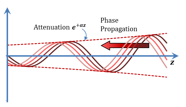
Figure 2.8

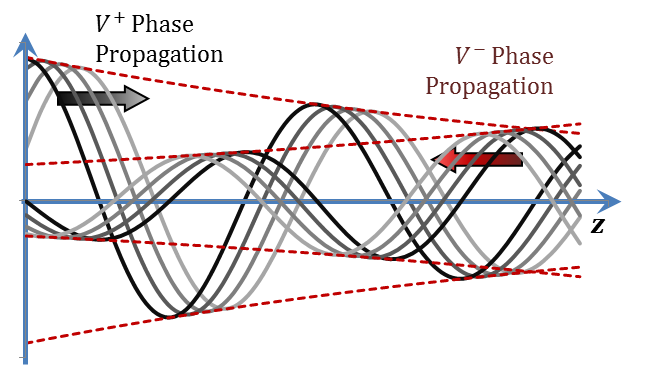
The two terms combined represent the $v\left( z,t \right)$ solution obtained in Equation (2.29). The complete solution is shown in Figure 2.9.

Figure 2.9

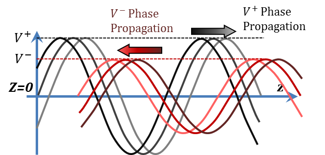
By the way, and before we leave this point, in the lossless TL case, the waves on the TL would not suffer any attenuation. The corresponding wave shapes are shown in Figure 2.10.

Figure 2.10

Physical Implications of Solutions - $\!~\gamma~\! ,~{{Z}_{o}},~{{V}^{+}},~and~{{V}^{-}}$:

Now as we saw the physical meaning of $\alpha$ and $\beta $, let us move back to the frequency domain solution in order to interpret the physical meaning of the parameters: $\!~\gamma~\! ,~{{Z}_{o}},~{{V}^{+}},$ and ${{V}^{-}}$.

$\!~\gamma~\! =\alpha +j\beta =\sqrt{\left\{ {{R}_{z}}+j\omega {{L}_{z}} \right\}\cdot \left\{ {{G}_{z}}+j\omega {{C}_{z}} \right\}}$
$\!~\gamma~\! $ is a complex quantity with real part $\alpha $ and an imaginary part $\beta $ .

The real part$,~\alpha ,$ appear in the exponent of the voltage and current solutions as to affect the amplitude of the wave along the TL (coordinate ${z}$). This real part becomes zero for lossless lines ${{R}_{z}}={{G}_{z}}=0$ and, hence, it is related with losses and causes the signals to attenuate as they travel along the line. For this reason, $\alpha $ will be called the attenuation coefficient, and its units are Nepers/meter.
$\left\{ One~Np~\left( Neper \right)=20/ln\left( 10 \right)~\cong 8.686~dB~\left( decibels \right) \right\}$

The imaginary part$,~\beta ,$ also appears in the exponent of the voltage and current solutions as to affect the phase of the wave along the TL (coordinate $z$). Hence, $\beta $ will be called the phase constant, and its units are radians/meter. For lossless lines, $\beta =\omega \sqrt{{{L}_{z}}{{C}_{z}}}$.

$\!~\gamma~\! $ is called the complex propagation constant of the TL.

${{Z}_{o}}={{R}_{o}}+j{{X}_{o}}=\sqrt{\left\{ {{R}_{z}}+j\omega {{L}_{z}} \right\}/\left\{ {{G}_{z}}+j\omega {{C}_{z}} \right\}}$

${{Z}_{o}}$ is a complex quantity with real part ${{R}_{o}}$ and an imaginary part ${{X}_{o}}$. For lossless lines, it reduces to a real value:
${{Z}_{o}}={{R}_{o}}=\sqrt{{{L}_{z}}/{{C}_{z}}}$

This may appear rather puzzling as we talk about a "Lossless" TL with ${{R}_{o}}$ equal to so many Ohms, e.g., a cable TV TL has a characteristic impedance of 75 Ohms. The thing is that there are no 75 Ohms resistor(s) in existence anywhere on this line and the 75 Ohms does not represent its internal resistance. It simply means that the 75 Ohms is nothing but a characteristic number representing the ratio between the traveling voltage and current waves.

${{Z}_{o}}$ is called the characteristic impedance of the TL.

It is worthy to note that both ${{Z}_{o}}~$and$~\!~\gamma~\! $ fully characterize the TL model. Given ${{Z}_{o}}~$and$~\!~\gamma~\! $ and using Equations (2.24) and (2.25), the RLCG model for the TL can be fully determined.

While both ${{Z}_{o}}~$and$~\!~\gamma~\! $ are characteristic parameters of the TL, ${{V}^{+}},$ and$~{{V}^{-}}$ are not. ${{V}^{+}}=\left| {{V}^{+}} \right|{{e}^{j\varphi _{v}^{+}}}$ , and ${{V}^{-}}=\left| {{V}^{-}} \right|{{e}^{j\varphi _{v}^{-}}}$ are two arbitrary constants that resulted from solving the TL differential equation without applying the boundary conditions, B.C. These constants can be fully determined once the TL conditions at its boundaries $(𝓏=0~$and$~at~𝓏 =ℓ)$ are implemented.

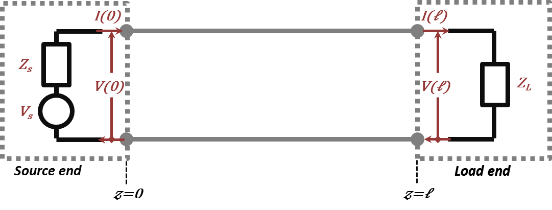
Figure 2.11

Referring to Figure 2.11, the boundary conditions, B.C., at the Source end are:

$V\left( 0 \right)={{V}^{+}}+{{V}^{-}}={{V}_{s}}-{{Z}_{s}}\cdot I\left( 0 \right)={{V}_{s}}-{{Z}_{s}}\cdot \frac{1}{{{Z}_{o}}}\left( {{V}^{+}}-{{V}^{-}} \right)$,

and the B.C. at the Load end are

$V\left( \ell \right)={{V}^{+}}{{e}^{-\!~\gamma~\ell }}+{{V}^{-}}{{e}^{+\!~\gamma~\ell }}={{Z}_{L}}\cdot I\left( \ell \right)={{Z}_{L}}\cdot \left\{ \frac{1}{{{Z}_{o}}}\left( {{V}^{+}}{{e}^{-\!~\gamma~\ell }}-{{V}^{-}}{{e}^{+\!~\gamma~\ell }} \right) \right\}$

These are two "complex variable" equations that can be solved to yield both ${{V}^{+}}$ and ${{V}^{-}}$ (magnitudes and phases). The resulting expressions can be written in the form:

${{V}^{+}}=\left\{ \frac{{{V}_{s}}~{{Z}_{o}}}{{{Z}_{s}}+{{Z}_{o}}} \right\}\left\{ \frac{1}{1-\left( \frac{{{Z}_{s}}-{{Z}_{o}}}{{{Z}_{s}}+{{Z}_{o}}} \right)\left( \frac{{{Z}_{L}}-{{Z}_{o}}}{{{Z}_{L}}+{{Z}_{o}}} \right){{e}^{-2~\gamma ~\ell }}} \right\}\tag{2.41}$

${{V}^{-}}={{V}^{+}}\left( \frac{{{Z}_{L}}-{{Z}_{o}}}{{{Z}_{L}}+{{Z}_{o}}} \right){{e}^{-2~\gamma ~\ell }}\tag{2.42}$

Physically, these are the levels of the waves travelling on the line. As will be discussed later, the ${{V}^{+}}$ is the level of the voltage wave traveling in the positive $z$ direction, while the ${{V}^{-}}$ is that of the negative $z$ wave. Considering that we only have one source of power (at the source end), there is only one explanation for the presence of a negative $z$ traveling wave; that it must have resulted as a result of waves reflecting (bouncing back) from the load end. A useful analogy here is watching the water waves at the seashore. The sea is the source of water that travels towards the shore. After the water waves hit the shore, we notice water waves traveling from the shore back to the sea. These are reflections of the original sea waves.

Video

1. In which direction does the voltage wave $\{1.8\ exp\ [-0.1z+j(3.77\times {{10}^{9}}t-18.13\ z)]\}$ propagate ($+z$ or $-z$)? What are the values of each of the attenuation coefficient and the phase constant? (Hint: Examine the real part of voltage wave expression). 
2. What would be the expression for this wave (Exercise 1) if it was to propagate in the opposite direction with no decay. 
3. What is the phase velocity for a lossless TL having $L_z=2.5~uH/m$, $C_z=500~pF/m$? 

Return to Lesson

Return to Video

1. Given a TL with the following per unit length RLCG model parameters: $R_z=0.01~Ohm/m$, $L_z=-0.5~uH/m$, $C_z=0.1~uF/m$, $G_z=1~mS/m$. At an operating frequency of $f=3~GHz$, find the attenuation coefficient, the phase constant and the characteristic impedance. 
2. Consider the circuit given in figure 2.11 consisting of a TL having the same parameters as in the previous example, a voltage source ${{V}_{s}}=2\ V$, $Z_s=50~Ohm$ and $Z_L=50~Ohm$. Find the value of $V^+$ and $V^-$ at $z=0$ and $z=4~cm$.

Return to Lesson

Return to Video

1. For Example 2 above, plot the magnitude of each of the individual voltage components $V^+(z)$, $V^-(z)$ and their sum over the length of the transmission line $(0\ to\ 4\ cm)$.
2. For the same Example 2 above, plot the magnitude of the ratio $V^+(z)/V^-(z)$ over the length of the transmission line. 
3. Repeat Problems 1&2 above while changing the parameters $L_z$ and $C_z$ to $12.5~\ uH/m$ and $0.005~\ uF/m$, respectively. Comment on the difference. 

Return to Lesson

Return to Video

Click here to download the Instructor Guide >>